TMM4175 Polymer Composites
Plane stress
A material is said to be under plane stress if the stress vector is zero across a particular surface. The assumption of plane stress simplifies the analysis considerably, and is an approximation that is typically made when analysing thin plates and shells.
Example: The hoop stress of a thin-walled cylinder subjectet to internal pressure $P$ is often approximated to $$ \sigma_h = \frac{PR}{t} $$
where $R$ is the radius and $t$ is the wall thickness. Considere the following parameters: $R_i=100$, $t=5$ and $P=10$ :
Ri, t, P = 100, 5, 10
print('Hoop stress for R = Ri     :', P*Ri/t)
print('Hoop stress for R = Ri+t/2 :', P*(Ri+t/2)/t)
print('Hoop stress for R = Ri+t   :', P*(Ri+t)/t)
Furthermore, we know intuitively that the radial stress $\sigma_r$ is equal to the negative of the internal pressure $P$ at the inside of the cylinder and zero at the outside of the cylinder.
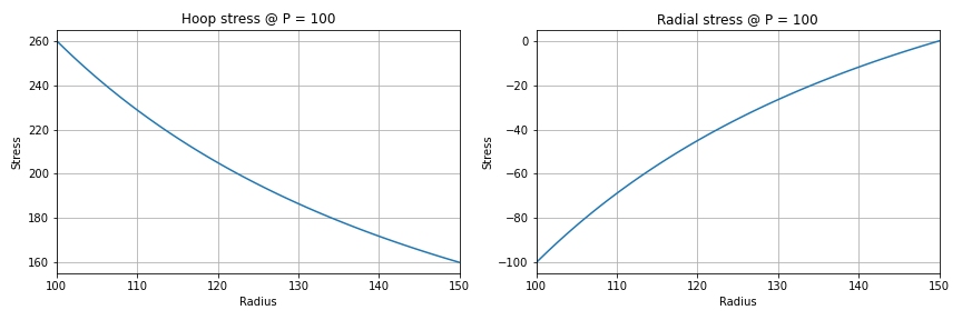
The exact solutions for a thick-walled cylinder of an isotropic material are
$$ \sigma_h = \frac{(R_i/R_o)^2+(R_i/R)^2}{1-(R_i/R_o)^2}P, \quad \sigma_r = \frac{(R_i/R_o)^2-(R_i/R)^2}{1-(R_i/R_o)^2}P $$import numpy as np
import matplotlib.pyplot as plt
%matplotlib inline
Ri, Ro, P = 100, 105, 10
R=np.linspace(Ri,Ro,11)
sigh = (((Ri/Ro)**2 + (Ri/R)**2)/(1-(Ri/Ro)**2))*P
sigr = (((Ri/Ro)**2 - (Ri/R)**2)/(1-(Ri/Ro)**2))*P
fig,(ax1,ax2)=plt.subplots(nrows=1,ncols=2,figsize=(12,4))
ax1.plot(R,sigh)
ax1.set_xlim(Ri,Ro )
ax1.set_xlabel('Radius')
ax1.set_ylabel('Stress')
ax1.set_title('Hoop stress')
ax1.grid(True)
ax2.plot(R,sigr)
ax2.set_xlim(Ri,Ro )
ax2.set_xlabel('Radius')
ax2.set_ylabel('Stress')
ax2.set_title('Radial stress')
ax2.grid(True)
plt.tight_layout()
plt.show()

The validity, or accuracy of using the plane stress assumption must obviously be made for the specific problem and structure in question. The previous example demonstrates that if the ratio of thickness to radius is small, the error made using thin-walled approximation is minor.
However, as the thickness to radius ratio increases, the radial stress cannot be ignored and the thin-walled approximation does not provide a reasonable result for the hopp stress as illustrated in the following figure:
Composites are often found as relatively thin plates and shells, which suggest that the plane stress assumption can be sufficiently accurate, at least on the larger scale. However, detailed 3-dimensional state of stress analysis must often be supplemented at joints, transitions and boundaries of the shell structure.
Hooke's law for an orthotropic material is
\begin{equation} \begin{bmatrix} \varepsilon_1 \\ \varepsilon_2 \\ \varepsilon_3 \\ \gamma_{23} \\ \gamma_{13} \\ \gamma_{12} \end{bmatrix} = \begin{bmatrix} S_{11} & S_{12} & S_{13} & 0 & 0 & 0 \\ S_{12} & S_{22} & S_{23} & 0 & 0 & 0 \\ S_{13} & S_{23} & S_{33} & 0 & 0 & 0 \\ 0 & 0 & 0 & S_{44} & 0 & 0 \\ 0 & 0 & 0 & 0 & S_{55} & 0 \\ 0 & 0 & 0 & 0 & 0 & S_{66} \end{bmatrix} \begin{bmatrix} \sigma_1 \\ \sigma_2 \\ \sigma_3 \\ \tau_{23} \\ \tau_{13} \\ \tau_{12} \end{bmatrix} \tag{1} \end{equation}Assume now that the stress vector is zero across surfaces with normals alligned with the 3-axis. This assumption implies that the non-zero stresses exist only in the 1-2 plane, i.e.,
\begin{equation} \sigma_3 = \tau_{23} = \tau_{13} = 0 \tag{2} \end{equation}The set of equations (1) can therfore be reduced to
\begin{equation} \begin{bmatrix} \varepsilon_1 \\ \varepsilon_2 \\ \gamma_{12} \end{bmatrix} = \begin{bmatrix} S_{11} & S_{12} & 0 \\ S_{12} & S_{22} & 0 \\ 0 & 0 & S_{66} \end{bmatrix} \begin{bmatrix} \sigma_1 \\ \sigma_2 \\ \tau_{12} \end{bmatrix} \tag{3} \end{equation}where the compliance matrix expressed by the enginering constants is
\begin{equation} \mathbf{S}=\begin{bmatrix} 1/E_1 & -\nu_{12}/E_1 & 0 \\ -\nu_{12}/E_1 & 1/E_{2} & 0 \\ 0 & 0 & 1/G_{12} \end{bmatrix} \tag{4} \end{equation}Implementation of a function for the 2D compliance matrix:
import numpy as np

def S2D(m):
    return np.array([[        1/m['E1'], -m['v12']/m['E1'],          0],
                     [-m['v12']/m['E1'],         1/m['E2'],          0],
                     [                0,                 0, 1/m['G12']]], float)
The 2D stiffness matrix of the material is simply the inverse of the compliance matrix:
\begin{equation} \mathbf{Q} = \mathbf{S}^{-1} \tag{5} \end{equation}In the following implementation we call the previous function for the compliance matrix S with a material (m) as argument. Then, the inverse of the compliance matrix S is returned:
def Q2D(m):
    S=S2D(m)
    return np.linalg.inv(S)
Example:
import matlib
m1=matlib.get('Carbon/Epoxy(a)')

Q=Q2D(m1)
print('Plane stress stiffness matrix:')
print()
print(np.round(Q))
Observe that the components of Q is not equal to the corresponding components of C
from compositelib import C3D
C=C3D(m1)
print(np.round(C))
print(Q[0,0]/C[0,0])
print(Q[0,1]/C[0,1])
print(Q[1,1]/C[1,1])
print(Q[2,2]/C[5,5])
The 2D transformation matrices are obtained by reducing the 3D transformation matrices for roation about the 3-axis:
\begin{equation} \mathbf{T}_{\sigma}=\begin{bmatrix} c^2 & s^2 & 2cs \\ s^2 & c^2 & -2cs \\ -cs & cs & c^2-s^2 \end{bmatrix} \tag{6} \end{equation}and \begin{equation} \mathbf{T}_{\epsilon}=\begin{bmatrix} c^2 & s^2 & cs \\ s^2 & c^2 & -cs \\ -2cs & 2cs & c^2-s^2 \end{bmatrix} \tag{7} \end{equation}
Both functions created below takes the orientation angle $a$ as the only argument:
from math import cos,sin,radians

def T2Ds(a):
    c,s = cos(radians(a)), sin(radians(a))
    return np.array([[ c*c ,  s*s ,   2*c*s],
                     [ s*s ,  c*c ,  -2*c*s],
                     [-c*s,   c*s , c*c-s*s]], float)

def T2De(a):
    c,s = cos(radians(a)), sin(radians(a))
    return np.array([[   c*c,   s*s,     c*s ],
                     [   s*s,   c*c,    -c*s ],
                     [-2*c*s, 2*c*s, c*c-s*s ]], float)
Transformation of the 2D stiffness matrix is given by: \begin{equation} \mathbf{Q{'}} = \mathbf{T}_{\sigma}^{-1}\mathbf{Q} \mathbf{T}_{\epsilon} \tag{8} \end{equation}
The transformed stiffnes matrix has the components
\begin{equation} \mathbf{Q}'= \begin{bmatrix} Q_{xx} & Q_{xy} & Q_{xs} \\ Q_{xy} & Q_{yy} & Q_{ys} \\ Q_{xs} & Q_{ys} & Q_{ss} \end{bmatrix} \tag{9} \end{equation}The function Q2Dtransform which takes the material stiffness matrix $\mathbf{Q}$ and the orientation angle $a$ as arguments:
def Q2Dtransform(Q,a):
    return np.dot(np.linalg.inv( T2Ds(a) ) , np.dot(Q,T2De(a)) )
Example:
Q=Q2D(m1)
print(np.round(Q))
print()
Qt=Q2Dtransform(Q,60)
print(np.round(Qt))
Hooke's law expressed in the global coordinate system is written as
\begin{equation} \begin{bmatrix} \sigma_x \\ \sigma_y \\ \tau_{xy} \end{bmatrix}= \begin{bmatrix} Q_{xx} & Q_{xy} & Q_{xs} \\ Q_{xy} & Q_{yy} & Q_{ys} \\ Q_{xs} & Q_{ys} & Q_{ss} \end{bmatrix} \begin{bmatrix} \varepsilon_x \\ \varepsilon_y \\ \gamma_{xy} \end{bmatrix} \tag{10} \end{equation}Plane stress thermomechanical relations
In the material coordinate system of an orthotropic material:
\begin{equation} \boldsymbol{\sigma} = \mathbf{Q}(\boldsymbol{\varepsilon} - \boldsymbol{\alpha}\Delta T ) \tag{11} \end{equation}\begin{equation} \begin{bmatrix} \sigma_1 \\ \sigma_2 \\ \tau_{12} \end{bmatrix} = \begin{bmatrix} Q_{11} & Q_{12} & 0 \\ Q_{12} & Q_{22} & 0 \\ 0 & 0 & Q_{66} \end{bmatrix} \begin{bmatrix} \begin{bmatrix} \varepsilon_1 \\ \varepsilon_2 \\ \gamma_{12} \end{bmatrix} -\Delta T \begin{bmatrix} \alpha_1 \\ \alpha_2 \\ 0 \end{bmatrix} \end{bmatrix} \tag{12} \end{equation}In a transformed coordinate system:
\begin{equation} \boldsymbol{\sigma}' = \mathbf{Q}'(\boldsymbol{\varepsilon}' - \boldsymbol{\alpha}'\Delta T ) \tag{13} \end{equation}\begin{equation} \begin{bmatrix} \sigma_x \\ \sigma_y \\ \tau_{xy} \end{bmatrix} = \begin{bmatrix} Q_{xx} & Q_{xy} & Q_{xs} \\ Q_{xy} & Q_{yy} & Q_{ys} \\ Q_{xs} & Q_{ys} & Q_{ss} \end{bmatrix} \begin{bmatrix} \begin{bmatrix} \varepsilon_x \\ \varepsilon_y \\ \gamma_{xy} \end{bmatrix} -\Delta T \begin{bmatrix} \alpha_x \\ \alpha_y \\ \alpha_{xy} \end{bmatrix} \end{bmatrix} \tag{14} \end{equation}where
\begin{equation} \boldsymbol{\alpha}'= \mathbf{T}_{\varepsilon}^{-1} \boldsymbol{\alpha} \tag{15} \end{equation}


Disclaimer:This site is about polymer composites, designed for educational purposes. Consumption and use of any sort & kind is solely at your own risk.
Fair use: I spent some time making all the pages, and even the figures and illustrations are my own creations. Obviously, you may steal whatever you find useful here, but please show decency and give some acknowledgment if or when copying. Thanks! Contact me: nils.p.vedvik@ntnu.no www.ntnu.edu/employees/nils.p.vedvik
Copyright 2021, All right reserved, I guess.