TMM4175 Polymer Composites
CASE STUDY: Thin-walled pipes
Cylindrical pressure vessels and pressurized tubes, or pipes, are important industrial components. Composite vessels and pipes manufactured by filament winding are found in a wide range of applications, from low-pressure water pipeline system to high-pressure storage of natural gas and hydrogen. Laminated tubes with closed ends subjected to partial pressure can be analyzed using laminate theory when a few idealized assumptions are fulfilled:
- Thin-walled refers in general to a vessel having a relatively large radius to thickness ratio, typically 10 and above. However, what we may consider as thin-wall is rather a matter of accuracy, where a greater ratio implies greater accuracy.
- Edge effects are neglected, which is generally a reasonable assumption far from the ends. This assumption implies that the tube wall is uniformly loaded.
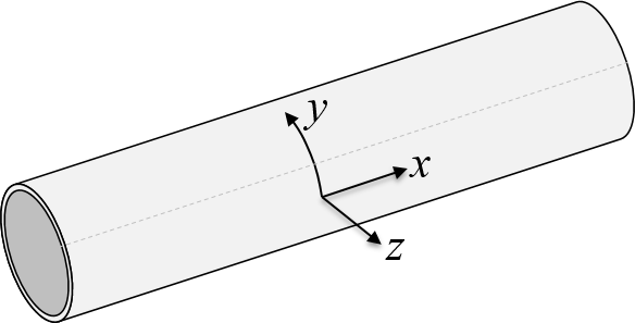
Consider a tube with closed ends having a radius R and subjected to a partial pressure P (the difference between inner and outer pressure). A coordinate system x,y,z defines the longitudinal direction (x), the hoop direction (y) and the normal to the cylindrical shell (z).
The section forces $N_x$ and $N_y$ are obtained by considering equilibrium in the two directions:
\begin{equation} \sum F_x = 0: \quad (N_x)(2\pi R) = (P)(\pi R^2) \Rightarrow N_x = \frac{PR}{2} \tag{1} \end{equation}\begin{equation} \sum F_y = 0: \quad (N_y)(2L) = (P)(2RL) \Rightarrow N_y = PR \tag{2} \end{equation}while the shear load $N_{xy}$ is zero in the absence of any torque loading on the tube. Note however that the shear strain can be different from zero according to relation (4) for a unbalanced laminate.
The curvatures are all zero due to the particular symmetry, which also implies that there will be internal moments for non-symmetrical layups. Hence the complete set of equations in the laminate theory framework is:
\begin{equation} \begin{bmatrix} N_x \\ N_y \\ 0 \\ M_x \\ M_y \\ M_{xy} \end{bmatrix} = \begin{bmatrix} A_{xx} & A_{xy} & A_{xs} & B_{xx} & B_{xy} & B_{xs} \\ A_{xy} & A_{yy} & A_{ys} & B_{xy} & B_{yy} & B_{ys} \\ A_{xs} & A_{ys} & A_{ss} & B_{xs} & B_{ys} & B_{ss} \\ B_{xx} & B_{xy} & B_{xs} & D_{xx} & D_{xy} & D_{xs} \\ B_{xy} & B_{yy} & B_{ys} & D_{xy} & D_{yy} & D_{ys} \\ B_{xs} & B_{ys} & B_{ss} & D_{xs} & D_{ys} & D_{ss} \end{bmatrix} \begin{bmatrix} \varepsilon_x^0 \\ \varepsilon_y^0 \\ \varepsilon_{xy}^0 \\ 0 \\ 0 \\ 0 \end{bmatrix} \tag{3} \end{equation}We can now split the set of equations into
\begin{equation} \begin{bmatrix} N_x \\ N_y \\ 0 \end{bmatrix} = \begin{bmatrix} A_{xx} & A_{xy} & A_{xs} \\ A_{xy} & A_{yy} & A_{ys} \\ A_{xs} & A_{ys} & A_{ss} \end{bmatrix} \begin{bmatrix} \varepsilon_x^0 \\ \varepsilon_y^0 \\ \gamma_{xy}^0 \end{bmatrix} \tag{4} \end{equation}and
\begin{equation} \begin{bmatrix} M_x \\ M_y \\ M_{xy} \end{bmatrix} = \begin{bmatrix} B_{xx} & B_{xy} & B_{xs} \\ B_{xy} & B_{yy} & B_{ys} \\ B_{xs} & B_{ys} & B_{ss} \end{bmatrix} \begin{bmatrix} \varepsilon_x^0 \\ \varepsilon_y^0 \\ \gamma_{xy}^0 \end{bmatrix} \tag{5} \end{equation}The latter equation is of no particular interest since the solution of (4) provides all we need for computing the layer results.
Computational example
A material:
import laminatelib
import matlib
m1=matlib.get('E-glass/Epoxy')
Layup:
layup1=[{'mat':m1, 'ori':-45, 'thi':1.0},
        {'mat':m1, 'ori':+45, 'thi':1.0}]
The submatrix A from the laminate stiffness matrix:
A=laminatelib.laminateStiffnessMatrix(layup1)[0:3,0:3]
print(A)
Radius, pressure and section forces:
R, P = 100, 2

Nx=P*R/2
Ny=P*R
Nxy=0
The laminate mid-plane strains:
import numpy as np
loads=[Nx,Ny,Nxy]
strains=np.linalg.solve(A,loads)
print(strains)
In order to use the function laminatelib.layerResults() we need the deformation as a 6x1 array:
deformations=np.concatenate((strains, [0,0,0]))
print(deformations)
res = laminatelib.layerResults(layup1,deformations)
For example, the stresses in the material coordinate system for the two layers:
res[0]['stress']['123']
res[1]['stress']['123']
Exposure factors for the layers:
res[0]['fail']
res[1]['fail']
Observe that the exposure factors are identical for both layers and position (top/bottom).
What is the optimum angle for a [-$\theta$/+$\theta$] laminate when the objective is to minimize the exposure factor given by the maximum stress criterion?
Solution:
def tubeResults(angle,R,P):
    layup =[{'mat':m1, 'ori':-angle, 'thi':1.0},
            {'mat':m1, 'ori':+angle, 'thi':1.0}]
    A=laminatelib.laminateStiffnessMatrix(layup)[0:3,0:3]
    loads=[P*R/2, P*R, 0]
    strains=np.linalg.solve(A,loads)
    deformations=np.concatenate((strains, [0,0,0]))
    res = laminatelib.layerResults(layup,deformations)
    return res
import matplotlib.pyplot as plt
%matplotlib inline

angles=np.linspace(0,90)
fE_MS = [tubeResults(angle,R=100,P=2)[0]['fail']['MS']['bot'] for angle in angles]
plt.plot(angles,fE_MS)
plt.grid(True)
plt.show()

Somewhere between 50 and 60. Limit the range:
angles=np.linspace(50,60)
fE_MS = [tubeResults(angle,R=100,P=2)[0]['fail']['MS']['bot'] for angle in angles]
plt.plot(angles,fE_MS)
plt.grid(True)
plt.show()

The failure pressure at the optimum angle is the applied pressure divided by the exposure factor:
fE_MS = tubeResults(53.5,R=100,P=2)[0]['fail']['MS']['bot']

print('Failure pressure for a 53.5 winding angle is',2/fE_MS, 'MPa')
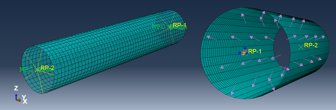
FEA model benchmarking
Briefly, a shell mode of a 1000 mm long tube with two layers oriented -53.5 and 53.5 relatively to the longitudinal axis. The ends are considered as rigid and the radius R=100 mm is to the mid-plane of the shell.
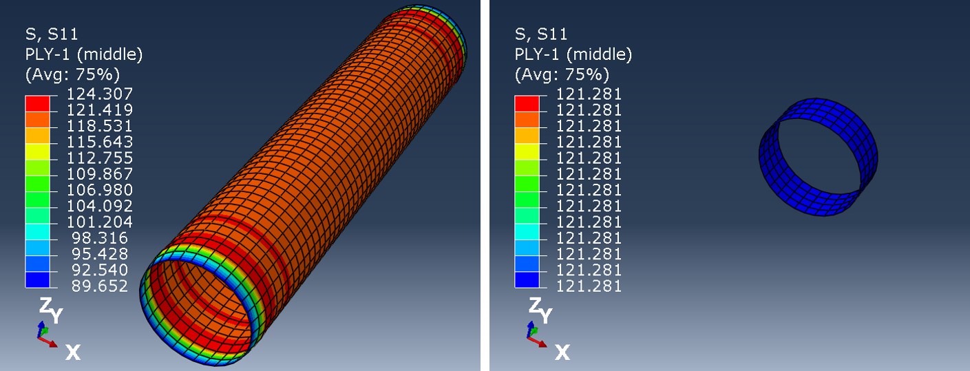
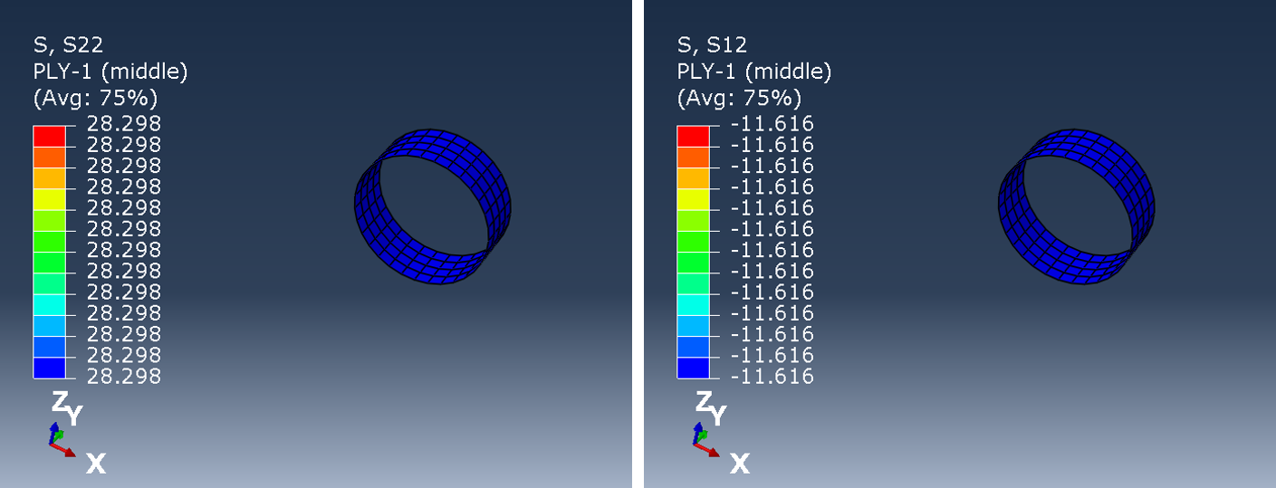
tubeResults(53.5,R=100,P=2)[0]['stress']['123']
The results do not compare well at regions close to the ends (top left figure), while the results far from the ends are, for all practial purposes, identical.
Disclaimer:This site is about polymer composites, designed for educational purposes. Consumption and use of any sort & kind is solely at your own risk.
Fair use: I spent some time making all the pages, and even the figures and illustrations are my own creations. Obviously, you may steal whatever you find useful here, but please show decency and give some acknowledgment if or when copying. Thanks! Contact me: nils.p.vedvik@ntnu.no www.ntnu.edu/employees/nils.p.vedvik
Copyright 2021, All right reserved, I guess.