TMM4175 Polymer Composites
CASE STUDY: Micromechanical finite element models
Finite element methods have been used extensively to predict the effective properties of fiber composites. The methods also enable detailed study of the stress distribution in the microstructure.
The following example demonstrates some of the principles on a simple (but not realistic) configuration: a square array of unidirectional fibers as illustrated in Figure-1.
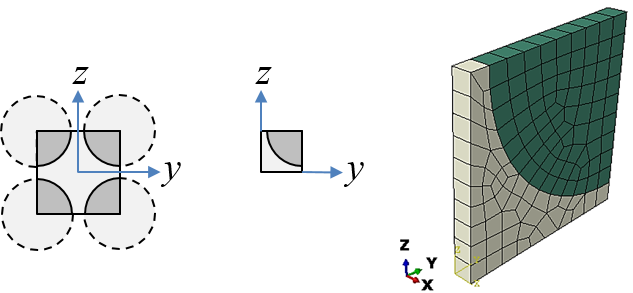
Figure-1: Square array of fibers and utilization of symmetry
A representative volume element (RVE) or unit cell, is a volume of the material exhibits statistically homogeneous material properties. For a repeating structure, the RVE is the smallest volume that can represent the whole structure (recall crystal systems and structures from basic material science courses)
The structure in Figure-1 is clearly orthotropic since we can identify 3 mutually perpendicular planes of symmetry. The constitutive relations for orthotropic materials are
\begin{equation} \begin{bmatrix} \sigma_1 \\ \sigma_2 \\ \sigma_3 \\ \tau_{23} \\ \tau_{13} \\ \tau_{12} \end{bmatrix}= \begin{bmatrix} C_{11} & C_{12} & C_{13} & 0 & 0 & 0 \\ C_{12} & C_{22} & C_{23} & 0 & 0 & 0 \\ C_{13} & C_{23} & C_{33} & 0 & 0 & 0 \\ 0 & 0 & 0 & C_{44} & 0 & 0 \\ 0 & 0 & 0 & 0 & C_{55} & 0 \\ 0 & 0 & 0 & 0 & 0 & C_{66} \end{bmatrix} \begin{bmatrix} \varepsilon_1 \\ \varepsilon_2 \\ \varepsilon_3 \\ \gamma_{23} \\ \gamma_{13} \\ \gamma_{12} \end{bmatrix} \tag{1} \end{equation}For simplicity, we will not consider the shear response. Since the normal strains are not coupled to the shear stresses, and normal stresses are not coupled to the shear strains, the set of equations is limited to:
\begin{equation} \begin{bmatrix} \sigma_1 \\ \sigma_2 \\ \sigma_3 \\ \end{bmatrix}= \begin{bmatrix} C_{11} & C_{12} & C_{13} \\ C_{12} & C_{22} & C_{23} \\ C_{13} & C_{23} & C_{33} \end{bmatrix} \begin{bmatrix} \varepsilon_1 \\ \varepsilon_2 \\ \varepsilon_3 \end{bmatrix} \tag{2} \end{equation}Due to the symmetry of the structure, it is now sufficient to model 1/4 of the RVE illustrated in Figure-1.
Consider a load case where the macro strains imposed on the RVE are
$$ \varepsilon_1,\varepsilon_2,\varepsilon_3=1,0,0 $$Through Hooke's law the effective stresses are
\begin{equation} \begin{bmatrix} \sigma_1 \\ \sigma_2 \\ \sigma_3 \\ \end{bmatrix}_{(1)}= \begin{bmatrix} C_{11} & C_{12} & C_{13} \\ C_{12} & C_{22} & C_{23} \\ C_{13} & C_{23} & C_{33} \end{bmatrix} \begin{bmatrix} 1 \\ 0 \\ 0 \end{bmatrix} \tag{3} \end{equation}Hence, one column of the effective stiffness matrix can be found by:
\begin{equation} \begin{bmatrix} C_{11} \\ C_{12} \\ C_{13} \end{bmatrix} = \begin{bmatrix} \sigma_1 \\ \sigma_2 \\ \sigma_3 \\ \end{bmatrix}_{(1)} \tag{4} \end{equation}We need two more load case for obtaining the other components of the stiffness matrix:
\begin{equation} \begin{bmatrix} \sigma_1 \\ \sigma_2 \\ \sigma_3 \\ \end{bmatrix}_{(2)}= \begin{bmatrix} C_{11} & C_{12} & C_{13} \\ C_{12} & C_{22} & C_{23} \\ C_{13} & C_{23} & C_{33} \end{bmatrix} \begin{bmatrix} 0 \\ 1 \\ 0 \end{bmatrix} \Rightarrow \begin{bmatrix} C_{12} \\ C_{22} \\ C_{23} \end{bmatrix} = \begin{bmatrix} \sigma_1 \\ \sigma_2 \\ \sigma_3 \\ \end{bmatrix}_{(2)} \tag{5} \end{equation}and
\begin{equation} \begin{bmatrix} \sigma_1 \\ \sigma_2 \\ \sigma_3 \\ \end{bmatrix}_{(3)}= \begin{bmatrix} C_{11} & C_{12} & C_{13} \\ C_{12} & C_{22} & C_{23} \\ C_{13} & C_{23} & C_{33} \end{bmatrix} \begin{bmatrix} 0 \\ 0 \\ 1 \end{bmatrix} \Rightarrow \begin{bmatrix} C_{13} \\ C_{23} \\ C_{33} \end{bmatrix} = \begin{bmatrix} \sigma_1 \\ \sigma_2 \\ \sigma_3 \\ \end{bmatrix}_{(3)} \tag{6} \end{equation}
The effective stresses are based upon volumetric averaging of the stress field $\boldsymbol{\sigma}$ in the micro structure:
\begin{equation} \bar{\boldsymbol{\sigma}}=\frac{1}{V} \int_V \boldsymbol{\sigma} dV \tag{7} \end{equation}Since the FEA is a discrete method, this translates to
\begin{equation} \bar{\boldsymbol{\sigma}}=\frac{1}{V} \sum_1^n \boldsymbol{\sigma}_i V_i \tag{8} \end{equation}where $n$ is the number of elements, $V$ is the total volume of the RVE, $V_i$ are element volumes and $\boldsymbol{\sigma}_i$ are element stresses.
The engineering constants for the composite can now be found by inverting the stiffness matrix and extracting the constants from the compliance matrix.
Accessing the results by scripting (Abaqus)
Note: The code that follows presume that Abaqus CAE is running, and that the output file (.odb) for the analysis has been opened.
# A variable (odb) pointing to the output database:
odb=session.odbs['C:/temp/TMM4175/cubearr1.odb']
# The sequence of volumes for each elements:
volumes= odb.steps['Step-1'].frames[-1].fieldOutputs['EVOL'].values
# The number of elements should be equal to the length of this sequence:
nelem=len(volumes)

# An array to store the stiffness matrix:
import numpy as np
C=np.zeros((3,3),float)

# Fore each load case (steps), compute the volume averageing stresses.
# Note that the stresses[i].data is an array of six values (data), while the
# volumes[i].data is a scalar value:
stresses=odb.steps['Step-1'].frames[-1].fieldOutputs['S'].values
for i in range(0,nelem):
    C[0,0] = C[0,0] + (stresses[i].data[0])*(volumes[i].data)
    C[1,0] = C[1,0] + (stresses[i].data[1])*(volumes[i].data)
    C[2,0] = C[2,0] + (stresses[i].data[2])*(volumes[i].data)

# Next: continue with the two other load cases...
# ...
# ...

# Then, divide the components by the total volume:

V = 100.0
C = C/V

# Finally, invert C and extract the engineering constants.
Results
Comparing the FEA results with the simple micromechanical models for different volume fractions:
Longitudinal modulus:
$$ E_1 = V_f E_{f1} + (1-V_f) E_m $$Transverse modulus:
$$ E_2 = \frac{E_{2f} E_m}{V_f E_m + V_m E_{2f} } $$Poisson's ratio:
$$ \nu_{12} = V_f \nu_{12f} + (1-V_f) \nu_m $$The dictionary of arrays called res is the results from finite element analyses.
import numpy as np

res={'v23': [0.45212599369943118, 0.42326753068320255, 0.38193586257143847, 0.32734263030771271, 0.26585209755220979],
     'Vf': [0.2, 0.3, 0.4, 0.5, 0.6],
     'v12': [0.31464432856635499, 0.29747797910557516, 0.28233369168316802, 0.26643119161704393, 0.25037967957843354],
     'v13': [0.31469489653996641, 0.29755840156758889, 0.28235464243866604, 0.26641034309063855, 0.25035627822974438],
     'E1': [16085.645326069418, 22933.106624840235, 29257.219022098543, 36080.085897475845, 42933.356895180361],
     'E3': [4645.4159028902841, 5820.2891324892262, 7340.3781020873903, 9686.6943935214549, 13329.110073619864],
     'E2': [4646.3660927156561, 5822.6259059409194, 7341.3386290148919, 9685.039457247738, 13325.605829518021]}

Vf=np.linspace(0.15,0.65,100)
E1f,E2f,Em,v12f,vm = 70000.0, 70000.0, 3000.0, 0.20, 0.35
E1mod = Vf*E1f + (1-Vf)*Em
E2mod = (E2f*Em)/(Vf*Em + (1-Vf)*E2f)
v12mod = Vf*v12f + (1-Vf)*vm

import matplotlib.pyplot as plt
%matplotlib inline

fig,(ax1,ax2) = plt.subplots(nrows=1,ncols=2,figsize=(12,4))
ax1.plot(Vf,E1mod, color='red',label=r'$E_1^{(Model)}$')
ax1.plot(Vf,E2mod, color='blue',label=r'$E_2^{(Model)}$')
ax1.plot(res['Vf'],res['E1'], 'x', color='red',label=r'$E_1^{(FEA)}$')
ax1.plot(res['Vf'],res['E2'], 'x', color='blue',label=r'$E_2^{(FEA)}$')
ax1.set_ylim(0,)
ax1.set_xlabel('Fiber Volume Fraction',size=12)
ax1.set_ylabel('Modulus [MPa]',size=12)
ax1.grid(True)
ax1.legend(loc='best')

ax2.plot(Vf,v12mod, color='green',label=r'$v_{12}^{(Model)}$')
ax2.plot(res['Vf'],res['v12'], 'x', color='green',label=r'$v_{12}^{(FEA)}$')
ax2.set_ylim(0,)
ax2.set_xlabel('Fiber Volume Fraction',size=12)
ax2.set_ylabel('Poissons ratio',size=12)
ax2.grid(True)
ax2.legend(loc='best')

plt.tight_layout()

Concluding remarks
- The simple models for longitudinal modulus and Poisson's ratio coincide well with the finite element results
- The transverse modulus predicted by the simple model does not compare well with the finite element results
- Note that the FEA model represents an orthotropic structure, but not a transversely isotropic.
- The relatively coarse mesh may have a minor influenc on the results.
Alternative configuration
Figure-2 shows an alternative configuration where the array of fibers is rotated 45 degrees about the $x$-axis.
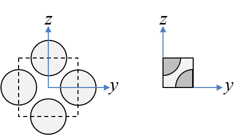
Figure-2: Square array of fibers, alternative configuration.
A study of this configuration will reveal significantly different results for the $E_2$ (left as an exersice). Results for the alternative configuration follows:
res = {'v23': [0.48705916463314547, 0.5025226793779568, 0.51191415645265204, 0.51834507152217246, 0.51786747853814974],
       'Vf': [0.2, 0.3, 0.4, 0.5, 0.6],
       'v12': [0.31616790203550948, 0.2976707843402604, 0.2825838970755265, 0.26773350324385864, 0.25052997460484572],
       'v13': [0.31618239036542367, 0.29759856352634556, 0.28254016445890251, 0.2677882872760769, 0.25050571739429789],
       'E1': [15499.556833602657, 22886.966365234468, 29163.538033952922, 35514.283106426003, 42853.027379392523],
       'E3': [4282.482584246075, 5014.7236761741196, 5782.595924314106, 6816.4386597434132, 8731.5794010146037],
       'E2': [4282.7143154182422, 5013.1670163681874, 5781.3518937291574, 6818.5939446495304, 8730.0204754334118]}

Vf=np.linspace(0.15,0.65,100)
E1f,E2f,Em,v12f,vm = 70000.0, 70000.0, 3000.0, 0.20, 0.35
E1mod = Vf*E1f + (1-Vf)*Em
E2mod = (E2f*Em)/(Vf*Em + (1-Vf)*E2f)
v12mod = Vf*v12f + (1-Vf)*vm

import matplotlib.pyplot as plt
%matplotlib inline

fig,(ax1,ax2) = plt.subplots(nrows=1,ncols=2,figsize=(12,4))
ax1.plot(Vf,E1mod, color='red',label=r'$E_1^{(Model)}$')
ax1.plot(Vf,E2mod, color='blue',label=r'$E_2^{(Model)}$')
ax1.plot(res['Vf'],res['E1'], 'x', color='red',label=r'$E_1^{(FEA)}$')
ax1.plot(res['Vf'],res['E2'], 'x', color='blue',label=r'$E_2^{(FEA)}$')
ax1.set_ylim(0,)
ax1.set_xlabel('Fiber Volume Fraction',size=12)
ax1.set_ylabel('Modulus [MPa]',size=12)
ax1.grid(True)
ax1.legend(loc='best')

ax2.plot(Vf,v12mod, color='green',label=r'$v_{12}^{(Model)}$')
ax2.plot(res['Vf'],res['v12'], 'x', color='green',label=r'$v_{12}^{(FEA)}$')
ax2.set_ylim(0,)
ax2.set_xlabel('Fiber Volume Fraction',size=12)
ax2.set_ylabel('Poissons ratio',size=12)
ax2.grid(True)
ax2.legend(loc='best')

plt.tight_layout()

Disclaimer:This site is about polymer composites, designed for educational purposes. Consumption and use of any sort & kind is solely at your own risk.
Fair use: I spent some time making all the pages, and even the figures and illustrations are my own creations. Obviously, you may steal whatever you find useful here, but please show decency and give some acknowledgment if or when copying. Thanks! Contact me: nils.p.vedvik@ntnu.no www.ntnu.edu/employees/nils.p.vedvik
Copyright 2021, All right reserved, I guess.