TMM4175 Polymer Composites

Home About Python Links Table of Contents

CASE STUDY: Elastic degradation of laminates¶

Problem statement¶

How does the effective modulus of a laminate changes due to transverse matrix cracks?

Consider a E-glass/epoxy laminate having the layup [0/90/0] where the thickness of the 90-oriented layer is twice a 0-oriented layer. When the laminate is subjected to a tensile load in the x-direction, initial failure will typically appeare as transverse matrix cracking running through the thickness of the 90-oriented layer as illustrated in Figure-1:

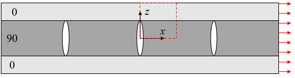
Figure-1

If we assume that the cracks are equally spaced, the problem can be reduced to the representative volume indicated in Figure-1 using symmetry and/or periodicity conditions at the boundaries.

FEA model¶

For simplicity, assume that the structure represents a laminate with infinite width (along the y-axis). In that case, it will be sufficient having only one solid element along this direction.

Dimensions of the representative volume: $\Delta x = 1$, $\Delta y = 0.05$, $t_{90} = 1$ where the relative crack distance for this case is

\begin{equation} c_d=\frac{2 \Delta x}{t_{90}} = 2 \end{equation}

Figure-2: Part, material and orientation

Mesh¶

As previously stated, one element along the y-direction will be sufficient. Linear element with reduced integration (C3D8R) will be prone to hour-glassing in this type of model, which is the reason for using elements of type C3D20R.

Figure-3: Mesh

Assembly and steps¶

The effective elastic properties $E_x,E_y$ and $\nu_{xy}$ can be obtained by solving for two load cases. These will be defined in two different steps, Step-1 and Step2.

Figure-4: Assembly and steps

Boundary conditions¶

The macro-strain of the unit cell for load step-1 and load step-2 shall be

\begin{equation} \begin{bmatrix} \varepsilon_x \\ \varepsilon_y \\ \end{bmatrix}_{(1)}= \begin{bmatrix} 1 \\ 0 \\ \end{bmatrix} \quad \text{and} \quad \begin{bmatrix} \varepsilon_x \\ \varepsilon_y \\ \end{bmatrix}_{(2)}= \begin{bmatrix} 0 \\ 1 \\ \end{bmatrix} \end{equation}

The consistent set of displacements maintaining macro-strains and symmetry conditions are shown in Figure-5 and Figure-6.

Figure-5: Boundary conditions for load case 1

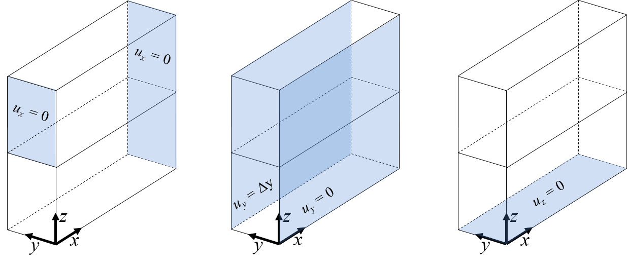
Figure-6: Boundary conditions for load case 2

Implementation:

Figure-7: Boundary conditions

Job and results¶

Figure-8: Job and results

Reaction forces¶

Figure-9: Extracting reaction forces

Effective laminate stresses from two load cases are found from the reaction forces normalized by respective cross section areas, and from the unit imposed unit strains we obtain the effective stiffness matrix components through Hooke's law:

\begin{equation} \begin{bmatrix} \sigma_x \\ \sigma_y \\ \end{bmatrix}_{(1)}= \begin{bmatrix} C_{11} & C_{12} \\ C_{12} & C_{22} \end{bmatrix} \begin{bmatrix} 1 \\ 0 \end{bmatrix} \Rightarrow \begin{bmatrix} C_{11} \\ C_{12} \end{bmatrix} = \begin{bmatrix} \sigma_x \\ \sigma_y \end{bmatrix}_{(1)} \end{equation}

and

\begin{equation} \begin{bmatrix} \sigma_x \\ \sigma_y \\ \end{bmatrix}_{(2)}= \begin{bmatrix} C_{11} & C_{12} \\ C_{12} & C_{22} \end{bmatrix} \begin{bmatrix} 0 \\ 1 \end{bmatrix} \Rightarrow \begin{bmatrix} C_{22} \\ C_{12} \end{bmatrix} = \begin{bmatrix} \sigma_x \\ \sigma_y \end{bmatrix}_{(2)} \end{equation}

import numpy as np

tot = 1.0
dx  = 1.0
dy  = 0.05

RF1_1 = 1.13251E+03
RF2_1 = 2.19148E+03

RF1_2 = 109.574
RF2_2 = 25.3122E+03

sigX_1 = RF1_1 / (dy*tot)
sigY_1 = RF2_1 / (dx*tot)

sigX_2 = RF1_2 / (dy*tot)
sigY_2 = RF2_2 / (dx*tot)

C = np.array( [[sigX_1, sigX_2],
               [sigY_1, sigY_2]])

S = np.linalg.inv(C)

Ex = 1/S[0,0]
Ey = 1/S[1,1]
vxy = - S[0,1]*Ex

print('Crack density = 2:')
print('Ex=',Ex)
print('Ey=',Ey)
print('vxy=',vxy)

Crack density = 2:
Ex= 22460.466014396217
Ey= 25100.16723250126
vxy= 0.08657801376411375

Comparing to undamaged and degraded laminate¶

import matlib, laminatelib
m = matlib.get('E-glass/Epoxy')

# Not degraded layers:

layup = [{'mat':m , 'ori': 0, 'thi':0.5},
         {'mat':m , 'ori':90, 'thi':1.0},
         {'mat':m , 'ori': 0, 'thi':0.5} ]

laminatelib.laminateHomogenization(layup)

{'E1': 25207.16112531969,
 'E2': 25207.16112531969,
 'v12': 0.11999999999999998,
 'G12': 3800.0,
 'a1': 1.0482142857142855e-05,
 'a2': 1.0482142857142859e-05}

from copy import deepcopy

md = deepcopy(m)

# Finding best fit factors:

md['E2']  = 0.43 * md['E2']      # reduced to 43%
md['v12'] = 1.0  * md['v12']     # not changed

# Degraded 90-layer:

layup = [{'mat':m ,  'ori': 0, 'thi':0.5},
         {'mat':md , 'ori':90, 'thi':1.0},
         {'mat':m ,  'ori': 0, 'thi':0.5} ]

laminatelib.laminateHomogenization(layup)

{'E1': 22442.59309331524,
 'E2': 25099.36382050038,
 'v12': 0.08636059853173003,
 'G12': 3800.0,
 'a1': 9.143831381392306e-06,
 'a2': 1.0232250672874081e-05}

Disclaimer:This site is about polymer composites, designed for educational purposes. Consumption and use of any sort & kind is solely at your own risk.
Fair use: I spent some time making all the pages, and even the figures and illustrations are my own creations. Obviously, you may steal whatever you find useful here, but please show decency and give some acknowledgment if or when copying. Thanks! Contact me: nils.p.vedvik@ntnu.no www.ntnu.edu/employees/nils.p.vedvik