4 An introductory session

Instead of analysing a real set of data, we will, to illustrates some of the possibilities of the library, first generate a simulated set of data from a known model. To do this let us first create a migration matrix using the steppingstone function. This function returns a stepping stone like $(n \times n)$ migration matrix of the following form

$$\mathbf{M} = (1-u) \begin{bmatrix}1-\frac12 m_0& \frac12 m_0& 0 &... ... & \ddots& \ddots & \ddots \\ & 0 & \frac12 m_0& 1-\frac12 m_0\\ \end{bmatrix},$$ (3)

which is what was used in Tufto et al. (1996). It takes two arguments; the first is the parameter vector theta (with elements representing $u$ and $m_0$), and the second is n, the number of subpopulations. Thus,

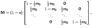
   > M <- steppingstone(c(.1,.2),10)

generates a migration matrix with $u=.1$ and $m_0=.2$, with dimension $(10 \times 10)$, that is,

> M
      [,1] [,2] [,3] [,4] [,5] [,6] [,7] [,8] [,9] [,10]
 [1,] 0.81 0.09 0.00 0.00 0.00 0.00 0.00 0.00 0.00  0.00
 [2,] 0.09 0.72 0.09 0.00 0.00 0.00 0.00 0.00 0.00  0.00
 [3,] 0.00 0.09 0.72 0.09 0.00 0.00 0.00 0.00 0.00  0.00
 [4,] 0.00 0.00 0.09 0.72 0.09 0.00 0.00 0.00 0.00  0.00
 [5,] 0.00 0.00 0.00 0.09 0.72 0.09 0.00 0.00 0.00  0.00
 [6,] 0.00 0.00 0.00 0.00 0.09 0.72 0.09 0.00 0.00  0.00
 [7,] 0.00 0.00 0.00 0.00 0.00 0.09 0.72 0.09 0.00  0.00
 [8,] 0.00 0.00 0.00 0.00 0.00 0.00 0.09 0.72 0.09  0.00
 [9,] 0.00 0.00 0.00 0.00 0.00 0.00 0.00 0.09 0.72  0.09
[10,] 0.00 0.00 0.00 0.00 0.00 0.00 0.00 0.00 0.09  0.81

In addition, let's assume that each subpopulation has effective size $N_e=100$ individuals. This is done by creating a vector Ne with elements specifying the effective size of each subpopulation:

   > Ne <- rep(100,10)
   > Ne
    [1] 100 100 100 100 100 100 100 100 100 100

We can now create some data by stochastic simulation using the simulate function. Required arguments are a matrix specifying the migration rates and the vector specifying effective populations sizes. If no additional optional arguments are given, a single vector of gene frequencies is returned:

   > simulate(M,Ne)
         [,1]  [,2] [,3] [,4]  [,5]  [,6]  [,7] [,8]  [,9] [,10]
   [1,] 0.285 0.315 0.44 0.61 0.655 0.495 0.495 0.46 0.575 0.425

M and Ne must, of course, have matching dimensions. To simulate data from more than one locus, the optional argument nloci should be given. A matrix of gene frequencies is then returned, where each row represent different loci. In this example, the returned matrix is stored in p:

   > p <- simulate(M,Ne,nloci=10)
   > p
        [,1]  [,2]  [,3]  [,4]  [,5]  [,6]  [,7]  [,8]  [,9] [,10]
  [1,] 0.520 0.455 0.505 0.640 0.730 0.715 0.455 0.560 0.630 0.515
  [2,] 0.635 0.535 0.485 0.530 0.610 0.450 0.370 0.415 0.515 0.510
  [3,] 0.535 0.375 0.295 0.355 0.475 0.570 0.715 0.610 0.665 0.660
  [4,] 0.615 0.555 0.535 0.550 0.485 0.565 0.470 0.475 0.325 0.465
  [5,] 0.390 0.440 0.445 0.435 0.550 0.510 0.385 0.385 0.610 0.650
  [6,] 0.705 0.580 0.490 0.410 0.565 0.480 0.565 0.745 0.750 0.755
  [7,] 0.445 0.365 0.340 0.475 0.575 0.670 0.640 0.635 0.580 0.585
  [8,] 0.490 0.395 0.545 0.395 0.310 0.320 0.390 0.325 0.280 0.250
  [9,] 0.705 0.625 0.570 0.610 0.410 0.460 0.395 0.335 0.245 0.145
 [10,] 0.320 0.300 0.400 0.255 0.320 0.450 0.440 0.425 0.495 0.295

In real life, one would typically load the gene frequency data matrix into R (or S-Plus) by doing something like:

   > p <- matrix(scan("data.txt"),byrow=T,nrow=10)

Using the approximation of the likelihood given in the appendix of Tufto et al. (1998), the maximum likelihood estimates of the parameters, for our simulated data set, can be found using the fitmodel function. This function takes two arguments; the name FUN of the migration model, and the gene frequency matrix:

   > fit1 <- fitmodel(steppingstone,p)

(The above call consumes about 33seconds of cpu-time on the SGI Indy unix box I have been using. With R running under Linux on a 90MHz Pentium processor it consumes about 25seconds. )

The $parameter component of the returned list contains the maximum likelihood estimates:

   > fit1$par
   [1] 0.004024386 0.128945698

and the $objective component contains the maximum likelihood:

   > fit1$obj
   [1] 125.4102

As illustrated by this example, the estimates obtained are, as they should, not excessivly far from the true values. If you sit down in front of your computer and actually do the above, you will of course get slightly different answers, which should come as any surprise, given that the data is random.

The fitmodel function is only a simple interface to, depending on whether you use R or S-plus, S-Plus' non-linear optimizer nlminb or R's nlm function. The list returned by nlminb or nlm is in both cases slightly modified so that the $objective component contains the maximum log likelihood and the parameter component contains the maximum likelihood estimates.