Brief Introduction to RO(C2)-graded cohomology
Representation spheres
For \(\small{G =C_2}\), the cyclic group of order two, any real representation \(\small{V}\) decomposes as
\[V \cong \mathbb{R}^{p,q} = (\mathbb{R}_{\text{triv}})^{\oplus p-q} \oplus (\mathbb{R}_{\text{sgn}})^{\oplus q}\]
where \(p\) is the topological dimension of \(\small{V}\) and \(q\) is the weight or twisted-dimension. We write
\(\small{S^V = S^{p,q}}\) for the representation sphere given by the one-point compactification of \(\small{V}\). Below are
some low-dimensional examples. Here \(\small{S^{1,1}}\) and \(\small{S^{2,1}}\) have the \(\small{C_2}\)-action given by
reflection across an equator and \(\small{S^{2,2}}\) has the \(\small{C_2}\)-action given by rotation about the axis through
the north and south poles.

For any virtual representation \(\small{V}\) and \(\small{C_2}\)-space \(\small{X}\), we write \(\small{H^{p,q}(X;\underline{\mathbb{F}_2})}\)
for the \(\small{RO(C_2)}\)-graded cohomology of \(\small{X}\) with coefficients in the constant \(\small{\mathbb{F}_2}\)-valued Mackey
functor.
The cohomology of a point
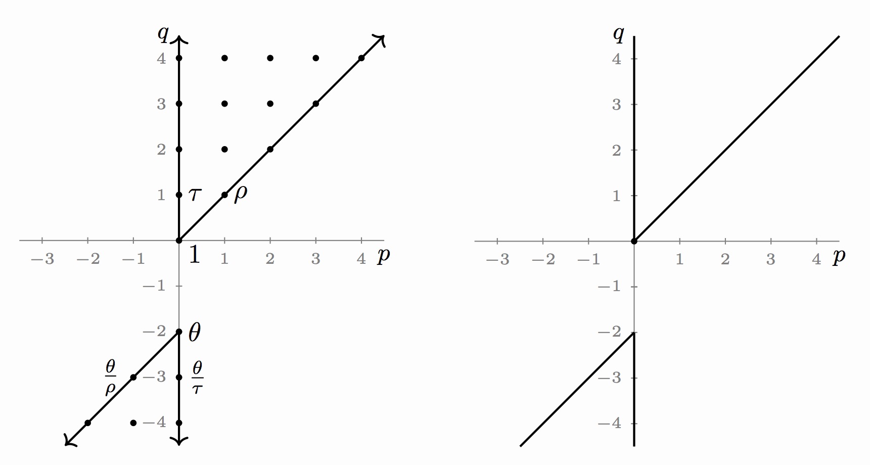
The bigraded cohomology of a point with the trivial action \(\small{\mathbb{M}_2 = H^{*,*}(pt;\underline{\mathbb{F}_2})}\)
is depicted below. A more detailed depiction is on the left, though it is often easier to work with the more succinct version on the right.
Here every lattice point inside the cones represents a copy of \(\small{\mathbb{F}_2}\). There are unique nonzero elements
\(\small{\rho \in H^{1,1}(pt)}\) and \(\small{\tau \in H^{0,1}(pt)}\). The top cone of \(\small{\mathbb{M}_2}\) is the polynomial ring
\(\small{\mathbb{F}_2[\rho,\tau]}\). The bottom cone has a unique nonzero element \(\small{\theta \in H^{0,-2}(pt)}\), which is
infinitely divisible by both \(\small{\rho}\) and \(\small{\tau}\), and satisfies \(\small{\theta^2=0}\).
Examples
For any \(\small{C_2}\)-space \(\small{X}\), there is always an equivariant map \(\small{X \to pt}\). This makes the \(\small{RO(C_2)}\)-graded
cohomology \(\small{H^{*,*}(X;\underline{\mathbb{F}_2})}\) into a bigraded \(\small{\mathbb{M}_2}\)-module. For example, let \(\small{S^n_a}\)
be the \(n\)-dimensional sphere with the antipodal action. Its cohomology as an \(\small{\mathbb{M}_2}\)-module is shown below. Again a
more detailed depiction is on the left and a more succinct version is on the right. Diagonal lines represent multiplication by
\(\small{\rho}\) and vertical lines represent multiplication by \(\small{\tau}\). As an \(\small{\mathbb{M}_2}\)-module
\(\small{H^{*,*}(S^n_a)} \cong \mathbb{F}_2[\tau,\tau^{-1},\rho]/(\rho^{n+1})\).

Up to equivariant isomorphism, there are six \(\small{C_2}\)-actions on the genus one torus. Their cohomologies as
\(\small{\mathbb{M}_2}\)-modules are depicted below. These computations were joint work with Eric Hogle.

Geometric representations
There are nice geometric representations of the elements \(\small{\rho}\), \(\small{\tau}\), and \(\small{\theta}\). By a theorem of dos Santos, we can represent
\(\small{H^{p,q}(-;\underline{\mathbb{F}_2})}\) by \(\small{K({\underline{\mathbb{F}_2}(p,q)) \simeq \underline{\mathbb{F}_2}\langle S^{p,q} \rangle}}\).
This is the usual Dold-Thom model of configurations of points on the representation sphere \(\small{S^{p,q}}\) with labels in \(\small{\mathbb{F}_2}\).
The basepoint in this model is a sink-source and when points collide their labels add. Both \(\small{\rho}\) and \(\small{\theta}\) factor as

where \(\small{\iota}\) is the canonical map sending each point \(\small{x}\) to the configuration \(\small{[x]}\). Here \(\small{\tilde{\rho}}\)
is the inclusion of the fixed-set, which is depicted below.
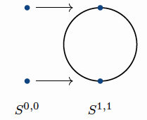
The map \(\small{\tilde{\theta}}\) is the quotient map. Finally, the element \(\small{\tau}\) can be viewed as a map
\(\small{S^{1,0} \to \mathbb{F}_2\langle S^{1,1} \rangle}\). In particular, \(\small{\tau}\) can be viewed as
a loop in the fixed set of \(\small{\mathbb{F}_2\langle S^{1,1} \rangle}\) as demonstrated by this
animation. The animation shows two particles that leave the sink-source,
travel symmetrically around \(\small{S^{1,1}}\), and then collide and disappear.