This document was made with assistance of Inf-HTML 0.9b (c) 1995 by Peter Childs
The file "ssiim14m.htm" is made from the OS/2 "ssiim.inf" file, using
the inf-html convertor made by Peter Childs. Some modifications are made
compared to the .inf file and compared to the User's Manual written in
WordPro, mostly with regards to graphics and equations.
A THREE-DIMENSIONAL NUMERICAL MODEL FOR SIMULATION OF SEDIMENT MOVEMENTS
IN WATER INTAKES WITH MULTIBLOCK OPTION
Version 1.4
The SSII model was developed in 1990-91 during the work with my dr. ing.
degree at the Division of Hydraulic Engineering at the Norwegian Institute
of Technology. SSII is an abbreviation for Sediment Simulation In Intakes.
The model was originally build around the numerical model Spider, which
was made by Prof. M. Melaaen during the work on his dr. ing. degree in
1989-90. Spider solves a flow problem for a general three-dimensional
geometry. SSII was made up of sediment calculation routines for 3D
solution of the convection-diffusion equation for the sediments,
communications with Spider and a graphical user interface made in OS/2.
The main motivation for making SSII was the difficulty to simulate fine
sediments in physical models. The fine sediments, often under 0.2 mm, are
important for wear on turbines. It was also an advantage to be able to
simulate other problems as for example sediment filling of reservoirs and
channels.
At the time SSII was made I had limited funding for computer equipment.
This, together with lack of knowledge of UNIX, made it necessary to
develop the models on a PC. Then a problem arouse, the 640 kB limit of
DOS. The arrays that the model used was often an order of magnitude larger
than the DOS limit. The DOS extenders were fairly unreliable at that time.
Because of the long computational times it was also important to have a
multi- tasking operating system. Therefore, the operating system OS/2 was
used. Compared to UNIX, OS/2 is much more user-friendly, and this has been
a major advantage during the development process, giving increased
productivity.
After finishing my dissertation in 1991, I wanted to improve the numerical
models. A disadvantage with the SSII and the Spider models for practical
situations was that a structured grid was used, and it was only possible
to have one block for an outblocked region. A natural improvement was a
multi-block model with general outblocking possibilities. This meant
considerable changes in Spider. Instead, a new water flow module for
multi-block calculation was made. This model was added to SSII, and the
resulting model was called SSIIM.
SSIIM, version 1.0, was uploaded on the Internet 17th of June 1993.
Version 1.1 had some bug-corrections and some improvements in the water
flow calculation for multiple blocks. Version 1.1 was uploaded on the net
18th of October 1993. In the fall of 1993 version 1.2 was made, with an
improved user interface, some additional tools and a revised manual. It
was uploaded on the net 22nd of December 1993. It was also distributed by
diskette to selected water institutions in January 1994. Version 1.3
included several bug-fixes, improved sediment calculation and improved
graphics. This was uploaded on the net 5th of April 1994. It took a while
until version 1.4 was uploaded on the net, mainly due to the OpenGL
additions. This meant that OS/2 version 4.0 had to be used. Version 1.4
also includes transient calculations of water flow, free surface and
sediment transport, water quality, a 2D depth-averaged water flow module
and improved graphics.
Future plans for SSIIM include a version with non-structured grid.
It is very likely that the graphics presentation modules will be improved.
There are also plans to include SSIIM in the River System Simulator (Internet:
www.sintef.no/nhl/rss/), a commercial product made by SINTEF Civil and
Environmental Engineering.
Several people have provided me with insight into the various problems I have encountered in the development of this program. I have benefitted greatly from the knowledge of Prof. Melaaen at Telemark Institute of Technology, in the science of computational fluid dynamics. In the topics of hydraulics and sedimentation engineering I have learned from Prof. Lysne at Division of Hydraulic and Environmental Engineering at the Norwegian University of Science and Technology, and from Prof. Julien, Prof, Gessler, Prof. Wohl and Prof. Bienkjewicz at Colorado State University. Knut Alfredsen helped me with software and hardware problems during the work with my dissertation, making the SSII model. Vijaya K. Singh at IBM Canada has helped me with the C compiler. Dave Zenz and Suzy Deffeyes at IBM Visual Systems has helped me with the OpenGL graphics. I would also like to thank the following people for helping me test the program: Morten Skoglund, Oscar Jimenez, Aslak Lvoll, Lars Abrahamsen, Siri Stokseth, J. Chandrashekhar, Knut Alfredsen, Hild Andreassen, Hilde Marie Kjellesvig, Md. Mahbubur Rahman, Tuva Cathrine Daae, Anne Sintic and Atle Harby. Also thanks to Richard Hibbert, Richard May, Luca Barone, Isabelle Lavedrine and Norbert Jamot at HR Wallingford Ltd, U.K. for their work and evaluation reports on SSIIM.
Trondheim, 7. May 1996
Nils Reidar Be Olsen
SSIIM is an abbreviation for Sediment Simulation In Intakes with
Multiblock option. The program is made for use in
River/Environmental/Hydraulic/Sedimentation Engineering. The main
motivation for the program is to simulate the sediment movements in
general river/channel geometries. This has shown to be difficult to do in
physical model studies for fine sediments.
The program solves the Navier-Stokes equations with the k-epsilon model on
a three-dimensional almost general non-orthogonal grid. The grid is
structured. A control volume method is used for the discretization,
together with the power-law scheme or the second order upwind scheme. The
SIMPLE method is used for the pressure coupling. The solution is implicit,
also over the boundary of the different blocks. This gives the velocity
field in the geometry. The velocities are used when solving the
convection-diffusion equations for different sediment sizes. This gives
trap efficiency and sediment deposition pattern.
The model has a graphicsl user interface with capabilities of presenting
plots of velocity vectors and scaler variables. The plots show a
two-dimensional view of the three- dimensional grid, in plan view, a
cross-section or a longitudinal profile. It is also possible to view the
geometry in three dimensions. Additionally it is possible to simulate
particle animation for visualization purposes.
Examples of graphics presentation for various cases
The model includes several utilities which makes it easier to give input
data. The most commonly used data can be given in dialog boxes. Several of
the modules in the program can be run simultaneously as separate threads.
This exploits the multi-tasking capabilities in OS/2. There is an
interactive graphical grid editor with elliptic and transfinite
interpolation. Grid and some of the input data can be changed during the
calculation. This can be useful for convergence purposes, and also when
optimizing the geometry with respect to the flow field.
Advice for new users are given, who also are recommended to try the
tutorial
SSIIM version 1.4 requires OpenGL graphics libraries to be installed with
OS/2. These are included in OS/2 version 4.0 and later. For earlier
versions, contact IBM to obtain the OpenGL libraries.
Some of the most important limitations of the program are listed below.
      * The program neglects non-orthogonal diffusive terms.
      * The program neglects stress terms for elements that are not at the
        boundary.
      * The grid lines in the vertical direction have to be completely
        vertical.
      * Internal walls cannot be used within two cells from a multi-block
        connection.
      * Kinematic viscosity and density of the fluid is equivalent to
        water at 20 degrees Centergrade. This is hard-coded and can
        not be changed.
      * Fully turbulent flow is assumed.

Also note that some combinations of different options may not have been
tested, and then there is a risk of a bug in the program. The animation
graphics routine is not maintained as well as the other routines, which
means that this routine has some bugs. The contour map graphics routine
also has a bug in connection with the boundary between blocks, and also
sometimes some contour lines are missing.
If you find any serious bugs that are not mentioned above, I would
appreciate if you let me know. You may use one of the following addresses:
E-mail:  Nils.R.Olsen@bristol.ac.uk
         Nils.R.Olsen@civil.sintef.no
         Nils.R.Olsen@bygg.ntnu.no
Ordinary mail:
Nils R. Olsen
SINTEF NHL
7034 Trondheim
Norway
I disclaim all warranties with regard to this software and the information
in this document, whether expressed or implied, including without
limitation, warranties of fitness and merchantability. In no event shall I
or my employer, SINTEF NHL, be liable for any special, indirect or
consequential damages or any damages whatsoever resulting from loss of
use, data or profits, whether in an action of contract, negligence or
other tortuous action, arising out of or in connection with the use or
performance of this software. It is therefore not recommended that the
program be used for solving a problem whose incorrect solution could lead
to injury to a person or loss of property. If you do use the program in
such a manner, it is at your own risk. It is necessary to know that to
understand and interpret the program results properly it is required that
the user have knowledge and experience in computational fluid dynamics and
hydraulic engineering.
If the user publish results where the SSIIM model has been used, the user
should include in the publication a statement that says that the SSIIM
model has been used.
Provided the user complies with the above statements, the program can be
used freely. The program can be distributed freely on condition that an
unchanged copy of this manual is distributed with the program.
Nils Reidar B. Olsen
Some of the theoretical basis is explained in this chapter. For more
details, including the equations, see the written manual or some of the
literature.
The initial water surface is generated by a standard one-dimensional
backwater calculation. The friction loss is calculated by Manning's
formula, using the friction factor given on the W 1 data set in the
control file. A separate Manning's friction factor for each cross- section
can be given on the W 5 data set. This prescribed water surface can
afterwards be changed according to the calculated pressure field. The
parameters for this procedure is given on the G 6 and the K 1  data set in
the control file. It is also possible for the user to specify the water
surface. This is done by setting the  K 1 data set in the control file to
K 1 0 0, and adding the vertical level of each grid intersection in the
koordina file. In this way it is possible to simulate for example a
tunnel.
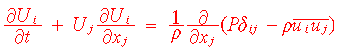
The Navier-Stokes equations for turbulent flow in a general three-dimensional geometry are solved to obtain the water velocity.
The k-epsilon model is used for calculating the turbulent shear stress.
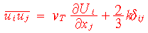
The Boussinesq approximation is used to solve the Reynold's stress term. The eddy-viscosity is given by:

Turbulent kinetic energy, k, is defined:

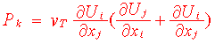
The differential equation for k is:
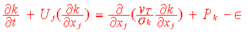
where Pk is given by:
The dissipation of k is called epsilon, and the equation solving for this parameter is:

The default algorithm in SSIIM neglects the transient term. To include
this in the calculations the F 33 data set in the control file  is used.
The time step and number of inner iterations are given on this data set.
For transient calculations it is possible to give the water levels and
discharges as input time series. The timei file is then used.
The gravity term is not included in the standard algorithms. It is however
invoked in some of the free surface calculations.
The equations are discretized with a control-volume approach. An implicit
solves is used, also for the multi-block option. The SIMPLE method is the
default method used for pressure-correction. The SIMPLEC method is invoked
by the K 9 data set in the control file. The power-law scheme or the
second-order upwind scheme is used in the discretization of the convective
terms. This is determined by the values on the  K 1 data set in the
control file. The numerical methods are further described in [3] and [4].
Wall laws for rough boundaries are used. These are given by Schlichting (1979).
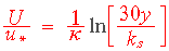
The roughness, ks, is equivalent to a diameter of particles on the bed. It can be specified on the F 16 data set in the control file. If the roughness varies at the bed, a roughness for each bed cell can be given in the bedrough file.
Influence of sediment concentration on the water flow
Note that there is still a discussion about the following arguments in the
science of sediment transport. Some of the explanations below are not
generally agreed upon.
The effect of the sediment concentration on the water flow can be divided
in two physical phenomena:
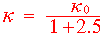
1. The sediment close to the bed move by jumping up into the flow and
settling again. This causes the water close to the bed to loose some of
its velocity, because some of the energy is used for moving the sediments.
This can be thought of as an added roughness. Einstein and Ning Chen [19]
conducted a set of classical experiments where they obtained a modified
velocity distribution as a function of the sediment concentration. This
function modifies kappa in the law wall.


This formula is coded in SSIIM,
and invoked automatically whenever the sediment concentration array has
values above zero, and the water flow calculation is done.
2. The other phenomena is that the sediment concentration increase the
density of the fluid, which changes the flow characteristics. A typical
example is a density current. This effect is added as an extra term in the
Navier-Stokes equations. This term is not automatically invoked. The user
can invoke this term by using the F 18 data set in the control file.
Note that the two effects will push the velocity profile in opposite
directions. Effect 1 will decrease the water velocity close to the bed,
while effect 2 will increase the water velocity close to the bed.
Sediment transport is traditionally divided in bedload and suspended load. The suspended load can be calculated with the convection-diffusion equation for the sediment concentration, c:
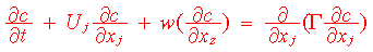
The fall velocity of the sediment particles is denoted w. The diffusion coefficient is taken from the k-epsilon model. The Schmidt number is set to 1.0 as default. If the user want a different number, this can be set on the F 12 data set in the control file.
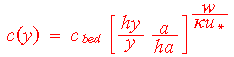
The concentration in the elements closest to the bed are found by various
methods described below. The concentration is "forced" on the bed boundary
finite volumes in a similar manner as the boundary condition for epsilon
in the k-epsilon model. The convection-diffusion equation is not solved
for the cells closest to the bed. Sediment continuity for these cells are
therefore usually not satisfied. The discrepancy in continuity is used to
calculate changes in the bed levels. This method also has the advantage of
simulating the interaction between the sediment that moves close to the
bed and the sediment that move in suspension.
Van Rijn [5] developed a formula for the equilibrium sediment
concentration close to the bed:
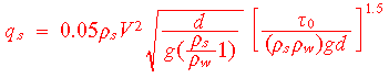
Another approach is to use a formula for total load, for example
Engelund/Hansen's [1] formula:


together with the theoretical vertical
sediment and water velocity distribution for uniform flow:
In SSIIM version 1.2 there were many different options for determining the
bed concentration. Since then a block-correction method has been added to
the sediment concentration solver. This meant a major improvement in
convergence, and also the difference between the various methods became
smaller. The choice of initial bed grain size distribution and
recalculation algorithm is given on the F 30 data set.
It is possible to calculate transient sediment transport. A transient term
is included in the differential equation. This algorithm is invoked on the
F 36 data set.
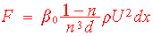
A roughness element in a complex geometry can always be modeled by
providing fine enough grid to dissolve the boundary of the roughness
element. The disadvantage with this method is that the number of grid
cells may be too excessive for practical use. Instead, the roughness
elements can be modeled within each grid cell. This can be done in two
ways, depending on the magnitude of the roughness elements. If the
magnitude is fairly small compared to the size of the grid cell, the
roughness can be incorporated in the law of the wall. If the roughness
elements are larger, other methods must be used. The porosity model used
in this study is developed by Engelund [20]:
Note that the porosity will also affect the turbulence in the flow field.
To model this it would be necessary to modify the k-epsilon turbulence
model. This is not done in this study. It is assumed that the source term
given by the porosity model is so great that it dominates over the
turbulent diffusive terms. Then the values of k and epsilon in the porous
domain will only have negligible effects on the flow field.
The porous domain is defined by the user for each cell as a distance above
the bed. The grid lines in the vertical direction is completely vertical
and parallel. This means that for each horizontal projection of the grid,
one must search for the cell where the top of the porosity is located.
Wall functions are applied in this cell, and the porosity model is applied
for the cells below. In the porous area the values for k are set to 0.01,
and the values for epsilon are set according to wall laws.
The porosity is calculated using a routine which is based on a set of
measured depths at different locations in the river. For each significant
rock in the river points are taken on top of the rock and on its sides.
Thus, several points are taken for each bed element. The porosity
generation model finds all the points in each bed cell, and calculates how
many points are located within certain elevations. The top elevation is
taken to be equal to the elevation of the highest point in the cell.
The porosity, pmin, at the bed level is given as a user input.
For each cell the porosity is calculated from interpolation from the set
of porosities as a function of the elevation.
The porosity calculation is further described in [12].
Calculations with porosity have to use a P on the F 7 data set in the
control file, and the porosity data must be given in the porosity file.
First, note that if a tunnel is simulated, and the user want to specify
the upper boundary, the K 1 data set in the control file should have the
parameter 0, and the koordina file should be arranged accordingly.
There are several methods of calculating free surface in SSIIM. The
standard (default) method is to use a one-dimensional backwater
calculation and use the result as a fixed lid with zero gradients.
Different Manning's friction factors can be given for the various
cross-sections on data set W 5 in the control file, thereby allowing the
user to make the appropriate lid.
The next alternative is to update the lid as a function of the calculated
pressure field. This is done on the G 6 data set in the control file. The
user gives which point in the grid that will not move, and the rest of the
surface grid moves according to the pressure field. This routine gives
satisfactory results for the curved channel example
There are two more alternatives, both coupled with the transient
calculation. The F 36 data set in the control file invokes the transient
free calculation. If the index is 2, than a routine similar to the routine
of the G 6 data set is used. This method is called method 2. The method
does not necessary give the correct flow field for a wave or a rapidly
moving surface. If the surface has only small movements, this method can
be used. Note that this method does not preserve water continuity.
If the index on the G 6 data set is 1, then another method is invoked.
 This method adds a gravity term in the Navier-Stokes equations. Thereby
the hydrostatic pressure field will result if the flow is uniform. The
movement of the water surface is based on the continuity defect in the
cells closest to the water surface. This is done instead of using the
SIMPLE algorithm for these cells. The method gives a more correct
simulation of rapidly moving water surfaces, as for example a flood wave.
Water continuity is satisfied, contrary to the other water surface
calculation methods. The disadvantage is that the calculation becomes more
unstable. This is further discussed here
The main user interface appears once the program is started and the input
files are read or generated.
If a control file is not present, the user is prompted for the necessary
parameters in a dialog box. A default control file is then made and
written to the disk.
If a koordina file is not present a rectangular channel is made initially.
A dialog box appears, which prompts the user for the length and the width
of the channel. The bed levels of the channel will be at elevation 0.0.
The water depth is given in the dialog box for the control file, or on the
W 1 data set in the control file.
The main user interface consists of a dialog box and a menu bar. The
dialog box appears in the lower left corner of the screen, and the menu
bar appears on the middle left side of the screen. The dialog box does not
have any editfields, only text fields and a push button. The dialog box
shows intermediate results. The two top lines in the dialog box are text
which is written from the different modules. There are also six numbers on
an exponential format. These are the residuals for the six equations in
the water flow calculation. The push-button is used for refreshing the
text and values in the dialog box.
The menu bar of the main user interface is used for starting different
sub-modules and showing graphics. The File option gives the possibility of
reading and writing different files. The Input Edit option gives the
possibility of editing the input data through a grid editor or dialog
boxes. The Computations option is used for starting the water flow or the
sediment calculations. The Graphics option is used for displaying the
results in different graphics windows.
Some of the most commonly used parameters can be set in dialog boxes.
These dialog boxes are activated by the Input Edit choice in the main menu
bar. The choices are:
* Grid Editor
* Sediment data: This gives the grain size, fall velocity and inflow of
each grain size. Note that the number of grain sizes can not be changed.
* Sediment parameters: This gives various parameters for calculation of
sediment flow.
* Waterflow parameters: This gives various parameters for calculation of
water flow. This is an important dialog box that is used when there are
convergence problems and when parameter tests are done. Note that the
parameters can be changed while the program is calculating the water flow
field.
Note that the parameters that can not be given in the dialog boxes have to
be given in the control file.
The grid editor is invoked by choosing GridEditor on the Input Edit
choice in the main menu. The user can click with the mouse on a grid
intersection and drag this to a new location. The mouse button must be
pushed down while the movement is made.
The main menu of the grid editor is made up of five main choices plus the
Help choice.
Move/Scale
Utility
Define
Generate
Note that after having edited the grid, it is advisable to write the
content to a koordina file. This is done in the File option of the main
menu. A file named koordina.new will be written. The attraction parameters
and the fixed point parameters can be written to the control.new file from
the same sub-menu.
The option Move is used to move the plot upwards, downwards or sideways.
The arrow keys can be used instead of the menu. The option Scale is used
to enlarge, shrink or distort the plot. The keys <Page Up> and <Page Down>
can be used for scaling. The option 2 Point Enlarge is used for enlarging
a certain section of the grid. After this choice is made, the user clicks
at the lower left corner and upper right corner of the part of the grid
that the user wants to see. After the second click the enlargement is
made.
The option Utility has five choices on the pull-down menu. The first
choice, Show geometrical points, displays the points in the geodata file
on the grid plot. The points are shown with a square, and the different
color indicate different vertical levels.
The second choice, Make bed interpolations, generates z values for the
bed surface of the grid. This is the same level as given in the koordina
file. This option can then be used to make the z values in the koordina
file, if the choice write koordina.new is made from the File option in the
menu of the main user interface. The bed interpolations are done in a
separate thread in OS/2, because the calculations may take some time. This
allows other tasks to be carried out during the interpolation.
The z values are interpolated from a set of geometrical data read from
the geodata file. If there is no geodata file present, an error message is
given. The interpolation routine goes through all the grid points i,j, and
finds the closest points in the geodata file in all four quadrants where
the grid intersection (i,j) is the center of the coordinate system. Then a
linear interpolation from these four points is made. If one of the points
in the geodata file is closer than 5 cm from the grid point, this z value
is chosen and no interpolation is done. The outcome of the interpolation
is logged to the file boogie.bed. If the interpolation routine is
unsuccessful in finding the point, the z value is set to zero.
The third choice, Apply changes, sets a global change flag. When the
waterflow routine sees that this flag is set it updates the calculation
geometry according to the grid editor geometry.
The fourth choice, Read koordina.mod, reads x,y and z values for one or
more points in the grid. The data in the koordina.mod file is on the same
format as in the ordinary koordina file, but it is not required that all
of the coordinates are present in this file. This option is useful if a
predefined shape is wanted, for example a circle. Then the grid line
intersections for the circle can be generated with a spreadsheet, and only
the points on the circle is placed in the koordina.mod file. When this is
read, the grid is moved according to the points on the circle.
The fifth choice, New water level and grid, is used after having changed
the z values on any of the coordinates. The grid editor only moves the
grid in the layer bordering the bed. So if any of the grid points have
been moved in the vertical direction, the water level and the grid points
above the bed needs to be recalculated. This is done by using this option.
Note that this will modify the koordina file according to the changes that
are made.
This option is used for defining different parameters. The parameters are
often connected to grid intersection points. The point that was last
activated by the mouse is used as default.
The first option is Give coordinates. This gives a dialog box where the
user can give numerical values for x,y and z for a grid intersection.
The second option is Set NoMovePoint. This invokes a mode where the user
can define certain points which will not be moved by the interpolation,
called NoMovePoints. In NoMovePoint mode it is not possible to move the
grid points with the mouse. When the user clicks on a grid intersection, a
blue star emerges on the intersection as a sign that this is chosen. Up to
200 NoMovePoints can be chosen. To verify that this mode is present, the
letters "Point mode, 0" is shown on the lower part of the editwindow when
the Set NoMovePoint is chosen. The integer shows how many points you have
chosen. To return to the normal mode, choose Define and Set NoMovePoint
again. It is verified that the normal mode is set because the text "Point
mode" disappears. In the normal mode the user can move all points
including the NoMovePoints.
The third option is Delete NoMovePoint. This deletes the last point set
under the NoMovePoint mode.
The following four options are setting of attraction to certain points or
lines in the grid. This is used by the elliptic grid generator. A dialog
box emerges when the choice is made, and the user must give two integers
which describes the location of the attraction point/line. Then two
attraction parameters are given. The Prop. att. value is proportional to
the attraction. If negative, the grid lines are moved away instead of
attracted. The Sq. att. value gives an attraction proportional to the grid
line difference raised to a power of Sq. att.. This value is used to
determine how far out in the grid the attraction works. Note that a
smaller value will give larger attractions. If the value of Prop. att. is
negative, the grid lines are moved away instead of attracted. Point
attraction gives attraction to points, and Line attraction gives
attraction to lines. Up to 200 attraction points can be defined. The
attraction points can be seen on the grid by colored rectangles at the
grid intersections.
The last option in the Define menu is Delete last attraction. This
deletes the last defined attraction.
The first choice in the pull-down menu is Boundary. This choice
interpolates linearly along the four border lines of the grid. Note that
the z values are also interpolated. This will create a rectangle unless a
NoMovePoint has been defined on the border. Then the interpolation will be
between the corners and the NoMovePoints.
The second choice is Elliptic. This starts the elliptic grid generator.
Note that this will not change the z values.
The third choice is TransfiniteI. This is transfinite interpolation in
the streamwise direction. The z values will be interpolated. In this mode
the NoMovePoints will also be moved.
The fourth choice is TransfiniteJ. This is the same as TransfiniteI,
except it is in the cross- streamwise direction.
The fifth choice is TransfiniteM. This is an average of TransfiniteI and
TransfiniteJ.
The sixth choice is Average. This is a procedure where the x,y and z
values of a grid intersection are taken to be the average of the four
neighboring grid intersections. This procedure is repeated for all the
inner grid intersections. This will not move the NoMovePoints.
Important notes:
1.    After having edited the grid, it is advisable to write the content
to a koordina file. This is done in the File option of the main menu. A
file named koordina.new will be written. The attraction parameters and the
fixed point parameters can be written to the control.new file from the
same sub-menu.
2.    Using unfavorable attraction coefficients can cause the elliptic
generator to crash, which means that SSIIM also crashes, and the grid data
are lost. It is therefore adviceable to write the grid to files before
starting the elliptic generation with attraction coefficients.
There are ten graphics modules for presentation of results. These can be
invoked any time during the calculation or afterwards. More than one
module can run simultaneously. The modules are choices under the Graphics
option of the main menu:
The modules use the standard GUI for OS/2, and have approximately the same
system of menus.
OpenGL 2D will show a two-dimensional projection of a profile in the x,y
or z plane. The profile will follow a grid surface. A cross-section will
be shown as a projection in the yz plane, a longitudinal profile will be
shown as a projection in the xz plane and a plan will be shown as a
projection in the xy plane. Also, the velocity vectors may not be parallel
to the grid. The x, y or z components is used.
The variables will be displayed with color shading. The colors will always
display red as the maximum value, then yellow, then green and blue as the
minimum value. The user can choose from a number of variables.
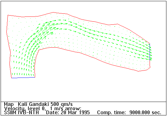
Examples of OpenGL plots are given in: Flow in a curved channel Map of
velocity field in a reservoir
OpenGL 3D shows an orthographic projection of grid surfaces. If no
surfaces are specified on the G 19 data set in the control file, the bed
of the geometry will be shown. Several G 19 data sets can be used to
specify three-dimensional surfaces of the geometry. The figure can be
rotated, scaled and moved. Various options for variables can be displayed.
Map presents the geometry seen from above. It is possible to get velocity
vector plots and plots and bar plots of concentration, diffusivity, k,
etc. It is also possible to plot the grid and change between different
vertical levels.
Contour map presents the variables as contour plots, seen from above. The
user can give the values of the contour lines on the L data set in the
control file. If the L data set is not given, seven contour lines will be
used. These are calculated to be within the range of the calculated
variable field. If the option Variable under Scale is chosen, the user can
give the numerical values of the lines. It is also possible to choose the
number of lines. Note that if more than 7 lines are chosen, all lines will
be black. Also note that if 0 lines are chosen in the dialog box, the
plotting will be similar to giving no L data set in the control file.
Color map presents the variables with colors and density patterns for each
cell depending on the value in the cell. This is seen from above. The user
can give different colors and shading pattern on the H data sets.
Longitudinal profile presents a longitudinal profile of the geometry.
Graphs with different parameters as a function of depth along the
longitudinal profile is obtained. It is also possible to view the grid or
the velocity vectors. It is possible to change between different
longitudinal profiles.
Cross-section presents a cross-section of the profile. It is only possible
to see a velocity vector profile. It is possible to change between
different cross-sections.
VerifyProfile presents calculated profiles of concentration or velocity at
locations specified by the user. It also presents user-given data in the
same plot. Arrange the measured values in the verify file.
VerifyMap presents calculated and measured velocity vectors in the same
figure. Different colors and legends are used to differentiate the
calculated and measured vectors. Arrange the measured values in the verify
file.
The purpose of the animation module is flow visualization. The module
displays the grid as seen from above, and animates the movement of a
sediment particle. The movement of the particle will depend on the flow
field and the fall velocity of the particle.
When the animation window starts, it checks a mouse scaling parameter. If
this is not provided in the G 15 data set in the control file, an X is
written in the window, and the user should click on this to make the
program scale the location of the mouse. If the user writes the
control.new file from the main menu, the correct G 15 data set is given in
this file.
The animation window has five menu options. These are Move and Scale which
are similar to the other presentation windows. Then there is the Particle
option. The pull- down menu is used to set the particle size, which will
be used by the program to calculate a fall velocity. The next menu option
is Run, which starts the particle movement.
The particle starts from one point in the grid and always from the top
cell in the vertical direction. Then it moves along the geometry until it
reaches one of the cells that borders the boundary. Then it returns to the
starting point. The starting point is changed by clicking with the mouse
at a location in the geometry.
The last option in the animation window menu is Speed. By choosing Double
or Half the time step is doubled or divided by two. This choice can be
repeated for further increase or decrease in time step. Note however that
if the time step becomes large, the particle may not move along the steam
lines any more, and it may even move out of the geometry during the time
step. The accuracy of the particle trajectory will increase with
decreasing time step.
The OpenGL graphics has an option Legend. This shows the color legend of
the plot. It can be used in presentations by using a screen-capturing tool
to move one of the legends to the word processor. The maximum and minimum
values are shown in the bar above the menu.
The OpenGL 2D graphics has an option Direction. This gives the choice of
displaying a cross-section, longitudinal profile or a plan view.
The OpenGL 3D graphics has an option Rotate. This gives the choice of
rotating the three-dimensional view around the x,y or z axis. Instead of
using the menu, it is possible to use the <F3> and <F4> keys to rotate
around the x-axis, the <F5> and <F6> keys to rotate around the y-axis and
the <F11> and <F12> keys to rotate around the z-axis.
The option Move is used to move the plot upwards, downwards or sideways.
The arrow keys can be used instead of the menu.
The option Scale is used to enlarge, shrink or distort the plot. The keys
<Page Up> and <Page Down> can be used for scaling. Some of the graphs also
use <CTL> + arrows for distorting the plot. The option 2 Point Enlarge is
used for enlarging a certain section of the grid. After this choice is
made, the user clicks at the lower left corner and upper right corner of
the part of the grid that the user wants to see. After the second click
the enlargement is made.
For the OpenGL plots, sub-menu under Scale can be used to move the color
scale to red or blue. This is also visualized in the Legend view. The <F7>
and <F8> keys can be used for the same purpose. For the OpenGL 2D plots,
the velocity vectors can be turned on/off and enlarged/shrinked. The <F5>
and <F6> keys enlarges/shrinks the velocity vectors.
The third option in the menu bar is Graph. The sub-menu displays different
parameters that can be shown. The option Sediment sample no. is a
reference to which of the N datasets from the control file is placed at
which location at the grid. The sub-menu option Bedchanges shows the bed
changes during and after sediment calculation. The sub-option Dominant
grain size shows which bed grain size has the highest fraction in each bed
element. The ColorMap option is be used for displaying a color map of some
of the following parameters: water depth, bed shear stress, turbulence,
velocity and sediment size. The colors are given by the user in the H data
sets in the control file.
The sub-option L-val concentration is used to change between different
grain sizes. When choosing Sum, the sum of the different grain sizes
(total concentration) is shown. The three last options are used for
changing which two-dimensional slice is presented. The two first sub-sub
options are i++, i--, j++, j--, k++, k--, depending on which direction is
changed. These options chooses the next(++) or previous(--) slice.
The next option on the menu bar is Timer. The timer is a module which
updates the graphics at certain time intervals. The numbers of the
different sub-options under Timer indicates the interval in seconds. The
options Start and End starts and stops the timer.
From the clipboard, the plot can be pasted directly into for example a
word processor that support the clipboard.
Also see Hardcopies
The last option on the menu bar is System or Save. The pull-down menu of
System has the option Save. This is used for storing the plot in an OS/2
metafile. It can then be printed or plotted on paper by the Picture Viewer
utility that comes with OS/2. The names of the metafiles file will be
mapfl000.met, longf000.met, color000.met, conto000.met, vprof000.met,
bedfl000.met or cross000.met, depending on which of the graphics
procedures that produced the file. If there is an existing file with the
same name, this will not be overwritten. Instead a new file with last
charachters 001 instead of 000 will be written. If this exist, further
increments in the number in the name will be made, until number 999.
Also see Hardcopies
The other options from System is Bedchange+ and Bedchange-. These options
only have effects in the Map graphics. The option Bedchange+ activates the
change in the bed levels according to the calculated bed changes.
Bedchange- changes the bedlevels back. It is not recommended to use these,
but instead use the time-dependent calculations that are introduced in
version 1.4.
It is not possible to plot directly from SSIIM to a plotter. One must
first make a graphics file, or copy to the clipboard, and then use a word
processor or a drawing program to plot to the plotter. Slightly different
techniques are used to make copies from the OpenGL plots and the other
plots.
Using the OpenGL graphics, it is necessary to use a screen capture utility
to make a copy to the clipboard or to make a bitmap file. This can for
example be done with the PmCamera utility, which is made by IBM. The
program is freeware and can be downloaded from internet sites. Start the
program in a separate window. PmCamera then gives a dialog box. Check on
the "active window" radiobutton, and on the "OS/2 Clipboard" checkbox.
Then minimize the dialog box with a click on the upper right icon. The
program will then run in the background and capture the graphics in the
active window. Next, run SSIIM, and display the OpenGL plot as you would
like to have the hard-copy. Then push the "PrintScreen" button on the
keyboard, and wait until you have heard two beeps. PmCamera has then
copied the graphics to the clipboard. It is also possible to let the
PmCamera utility make a bitmap file, which can be stored.
To plot the OpenGL graphics from the clipboard, one can for example use
the IBMWORKS wordprocessor from the Bonus-pack. Start the word-processor,
and choose "paste" from the "edit" of the menu to copy from the clipboard.
Then print the result.
Using non-OpenGL graphics, it is possible to copy directly to the
clipboard or to a metafile from SSIIM. It is then also possible to use a
word processor to copy from the clipboard, or import the metafile and then
print the results. A useful utility which is bundeled with OS/2 is
PicView, which plots the vector graphics from the clipboard or from a
metafile to the plotter.
Some advice when plotting on a pen plotter: If the lines of the plot are
not clear, leave the paper in the plotter and plot several times on the
same paper. This technique can also be used to get both vector and color
plots on the same figure.
most of the files are only used for special purposes and they are normally not required. Some of the files are output files. The program can produces many of the input files. For simpler cases all the necessary input files can be generated by the program. The two main input files are the control file and the koordina file. All the files are ASCII files, and can be created using a standard editor.
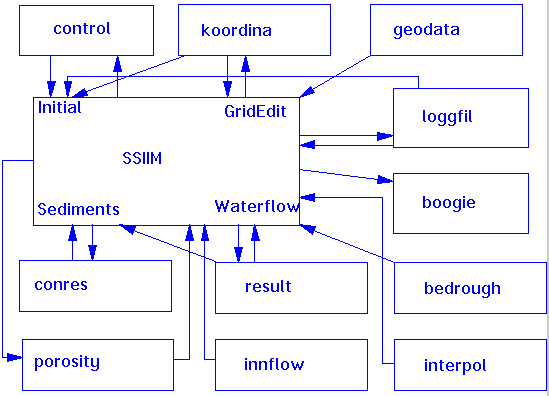
SSIIM file structure for main files
The control file gives most of the parameters the model needs except the
grid. The main parameters are the grid size, that is how many grid lines
there are in the three directions. The number of sediment sizes is also an
important parameter. To generate the water surface it is necessary to know
a downstream water level, together with the water discharge and the
Manning's friction factor. These parameters are given on the G 1 and the W
1 data set in the control file. If the control file does not exist, the
user is prompted for these parameters in a dialog box. The user can then
later choose Write control in the File option of the main menu, and get a
control file written to the disk (as control.new). This can then be edited
according to the user's needs. Note that only the most used parameters are
written to the control.new file.
During the water flow calculations there are several parameters that can
be varied. These parameters affect the accuracy and the convergence of the
solution. These parameters can be modified while the water flow field is
being calculated. A dialog box with the parameters is invoked by choosing
Waterflow parameters from the Input Editor choice in the main menu.
The control file contains all other data that are necessary for the
program. SSIIM reads each character of the file one by one, and stops if a
capital T,F,G,I,S,N,B or W is encountered. Then a data set is read,
depending on the letter. A data set is here defined as one or more numbers
or letters that the program uses. This can for example be the water
discharge, or the Manning's friction coefficient. It is possible to use
lower-case letters between the data sets, and it is possible to have more
than one data set on each line. Not all data sets are required, but some
are. Default values are given when a non-required data set is missing.
SSIIM controls the data sets in the control file to a certain degree, and
if an error is found, a message is written to the boogie file and the
program is terminated.
Remember that the order of the data sets may be important. For example
the G 1 data set should be early in the file. If the order of the data
sets follows the description given here, this should not be a problem.
For the initialization and graphics, the following data sets are
required:
G 1, G 3, W 1-2
For the sediment calculation, the following data sets are required:
S, I
For the water flow calculation by using MB-Flow, no data sets are
required.
In addition, there are a number of optional data sets for each
calculation. These are described below.
Title field. The following 30 characters are used in the graphics
Debugging possibility. If the character that follows is a D, one will get
a more extensive print-out to the boogie file. If the character is a C,
the coefficients in the discretized equations will be printed to the
boogie file.
Automatic execution possibility. Some parts of the program will be
executed directly after the initialization if a character is placed in
this field. The sub-programs will be executed in the order they are given.
The possibilities are:
 R Read the result file
 I Initialize the sediment calculations
 S Calculate sediment concentration
 W Start the multi-block water flow routine
 B Change the bed according to sediment calculation
 M Write result file
 V Initialize water surface level
Relaxation factor for second order interpolation of bed concentration,
maximum iterations for concentration calculations and convergence criteria
for suspended sediment calculation. The convergence criteria is given as
allowable flux deficit as part of inflowing sediments.
Defaults: relaxation: 0.5, iterations: 500, convergence criteria: 0.01.
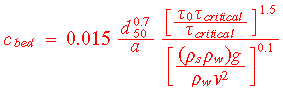
Coefficients for formula for bed concentration. Default is van Rijn's
coefficients: 0.015, 1.5 and 0.3. If one uses this option, the sediment
transport formula given in dataset F 10 must be R, which is van Rijn's
formula is used as basis.
Run options. read 10 characters. If the following capital letters are included this will mean:D Double the number of grid cells in streamwise direction in comparison to what is given in the koordina file. Each cell is divided in two equal parts. When this option is used for the whole geometry, the number of grid lines in the streamwise direction (on the G 1 data set) must be multiplied with 2 and 1 must be subtracted. J Double the number of grid cells in the cross-streamwise direction. The same procedure for the lines in the cross- streamwise direction (G 1 data set) is required. I Inflowing velocities in the y-direction are set to zero. A Diffusion for sediment calculations in non-vertical direction is set to zero. B Correction for sloping bed is used when calculating bed sediment concentration. G Cell walls at outblocked area is not changed when there are changes in the cells outside the block. V 90 degree turning of the plot seen from above (map). Z Vertical distribution of inflowing sediment is uniform. X Grid is read in from the "XCYC" file. This is only used in the post-processor, and with presentation of results from Spider where the lines in the k-direction are not vertical. C Inflowing and ouflowing water in default walls is set to zero. This means that the water flow must be specified on the G 7 data sets. P Use the porosity file
Maximum bed level change relative to water depth. This is controlled for
all the cells. Default: 0.1. This parameter is used to compute the time
step for the bed changes.
Factor that is used to change the turbulent viscosity of the inflowing
water. The factor is proportional to the turbulent viscosity. Default:
1.0.
Which sediment transport formula is used to calculate the concentration at
the bed. The following options are given:
 R van Rijn's formula
 E Engelund/Hansen's formula
 A Ackers/White's formula
 Y Yang's streampower formula
 S Shen/Hung's formula
Default: R.
Note that only the option R is fully tested.
Density of sediments and Shield's coefficient. Default: 2.65 and 0.047.
Schmidt's coefficient, which is a correction factor for deviation between
the turbulent diffusivity for sediment and water. Default: 1.0
An integer that determines how the law walls will be used in the cells
which borders both the wall and the bed. A value of 0 will make the
program use wall laws on both walls. A value of 1 will make the program
only use wall laws on the bed wall. For cases where the vertical
dimensions are approximately the same as the horizontal dimensions, a
value of 0 is recommended. Default: 0.
Roughness coefficient which is used on the side walls and the bed. If not
set, the coefficient is calculated from the Manning's friction
coefficient. The file bedrough overrides this value for the bed cells.
Time step in seconds. When this is above 10-8 a transient term is
included. Default 0.0 (non-transient calculations)
Density current source. A float is read, and if it is above 10-6, the
sediment density term in the Navier-Stokes equation is added. The float is
multiplied with the density term, so a value of 1.0 is recommended when
this term is needed. Default 0.0 (the term is not used).
Repeated calculation option. An integer is read, and the calculation
sequence on the F 2 data set will be repeated this many times. Note that
the graphical view of the bedlevel changes will only appear on the last
iteration when sediment calculations are done. Also note that if a result
file is read in the F 2 data set, it is only read during the first
iteration.
Relaxation coefficient for the Rhie and Chow interpolation. Normally a
value between 0.0 and 1.0 is used. When 0.0 is used the Rhie and Chow
interpolation will have no effect. When 1.0 is used the Rhie and Chow
interpolation will be used normally. Default 1.0.
Minimum porosity and relaxation factor for porosity calculations. Two
floats. Default 0.2 and 2.0.
Accelerated deposition routine. Two floats are read. The routine fills a
reservoir to a certain percentage of the total volume. This volume
fraction is given on the first float. The filling is based on only one
water flow calculation. Therefore the sediments may fill over the water
surface in some locations. The routine then moves away some sediments so
that a certain water depth is kept. This depth is given by the second
parameter, in meters. The surplus sediment is distributed to neighboring
cells according to the one water flow calculation. The redistribution is
iterated so that there are no filling above the minimum water depth.
Note that the bed changes are calculated in the center of the cells, and
that changes in the grid therefore are interpolated from four surrounding
cells. This means that even if the four surrounding elements are filled to
the given criteria, the grid line may not be exactly on this level. This
may cause bedlevels to rise above the waterlevel. The used should examine
the grid after the bed changes to observe whether this has occurred.
Choosing a higher value of the minimum water depth will decrease the
chance for such a phenomena to occur.  Also note that using this option
will not give the correct deposition pattern according to the hydraulics
of the reservoir. Also, sediment continuity may not be satisfied, if there
also are erosion in some part of the geometry.
Turbulence model. An integer is read, which corresponds to the following
 models:
 0 : standard k-* model (default)
 7 : eddy viscosity = 0.11 * depth * shear velocity (Olsen, 1991)
Note that only option 0 and 7 has been implemented, and that option 7
only works for the two-dimensional calculation.
Porosity parameters. Four floats and one integer. The two first floats are
identical to the ones on the F 22 data set. The following two floats give
the porosity on the second and third level above the ground. These have
default values 0.5 and 0.8. These are used if the roughness height is
larger than the levels of the porosity in the porosity file. The effective
porosity height is set to maximum of bed cell height and roughness height.
The last integer determines the procedure for finding particle diameter in
the porosity formula. The following options are given: (default 0)
 0 : Maximum of roughness height and porosity height
 1 : Maximum of roughness height and 0.33 * porosity height
 2 : Equal to height of bed cell
 3 : Maximum of height of bed cell and porosity height
Volume fraction of sediments in deposits. One float is read. Default 0.5.
If the water content is 51 % in a fully saturated sample, the volume
fraction will be 0.49.
If the accelerated deposition routine is used, the sediments depositing
over the given level below the surface have to be moved. This data sets
gives some of the data for where it is moved. Three integers and one
double are read. If the first integer is 1, the program will go through a
loop where the depositions in the most upstream elements will be averaged.
The following two integers are loop indexes that tells how many times the
program will pass through a loop which moves the depositions. The second
integer is for a loop which moves depositions equally in all directions,
called a diffusive moving. The third integer is for a loop which moves
depositions along the water flow direction, called a convective moving.
The last number, the float, tells how much of the deposits will be moved
by the diffusive movement. Note that the convective moving is invoked
before the diffusive moving.
Default: F 28 1 2 <n> 1.0
<n> = xnumber*ynumber*10
Bed concentration recalculation methods. Six integers are read. The first
integer determines which initial bed sediment grain size distribution is
present. The following possibilities are present:
 0 : Given by the user on the N data sets
 1 : Shield's graph method
 2 : Zero for all sizes
The second integer tells which method is used to recalculate the bed
 sediment grain size distribution. The following options are given:
 0 : No recalculation
 1 : Recalculation based on fluxes in/out of the bed cell
 2 : Recalculation based on deposition
 3-5 : Recalculation based on deposition and erosion
Option 3 and 4 does not necessarily scale the sum of the fractions to
unity, if the sum is below unity. Option 5 does. Option 4 allows the sum
of the fractions to be above unity, whereas option 3 and five does not.
Note that the method for recalculation of bed grain size distribution is
still on the experimental stage, and that the above options are not
verified yet.
The third integer invokes second order extrapolation of bed concentration
if it is 2.
If the fifth integer is 2, it invokes routine that keeps the bed
concentration under the level of the inflowing concentration.
Default: F 30 0 0 0 0 0 0 Note that six integers must be present, even if
only one or two are different from zero.
Two porosity coefficients are read. The coefficients are used for making
the porosity file. This is further described here  Default: F 31 0.8 0.8
Transient water flow parameters. A float and an integer is read. The float
is the time step. The integer is the number of inner iterations for each
iteration.
Transient free surface routine is invoked if the F 36 1 data set is
present. Note that this has not yet been fully implemented.
Transient sediment calculation is invoked if the F 37 1 data set is
present. Note that this has not yet been fully implemented.
Residual limit for when warning messages are written to the boogie file.
Default: 1.0e+7.
Turbidity current parameter. If this is unity the extra term in the
Navier- Stokes Equation are taken in that takes into account the effect of
gravitational forces on water that have higher density because of high
sediment concentration. If this is above 0.001, the term is still
incorporated but relaxed with the factor on the data set. Default 0.0.
Maximum scour depth for bed changes in meters.
Minimum level where the bed will not move under in meters.
Underflow parameter. An integer is read. If it is 1 the solver will check
for underflow errors and correct these. This procedure will cause SSIIM to
run slightly slower. The parameter can be used if the program halts with
the system underflow error. This is most often encountered when blocking
out regions of the flow. Default 0.
Two-dimensional flow calculation parameter. If 1 the two-dimensional
calculation will be used. If 0, the 3D calculation will be used. Default
0.
Transient Free Surface parameters. Three floats are read.
The first is a diffusion parameter for spreading of water flow elevation
to the corners of the cell. A small parameter will cause movements in the
direction of the flow. A larger value will give more movements in all
directions. It is only used when the flow is supercritical. Default 0.05.
The second float is an accelleration factor for speeding up a wave. When
zero, this has no effect. A factor of 1.0 may give higher speed. Default
0.0.
The third float is a damping parameter for obstacles in the flow. Default:
2.0, which means no damping.
Interpolation parameter in meters. One float is read, which is used in the
bed interpolation routine that are called from the GridEditor.  If the
points given in the geodata file are located a horizontal distance under
the interpolation limit, than the interpolation routine will use the exact
value of the geodata point instead of interpolating from surrounding
points. Default: 0.05 m.
Parameter for interpolation of results. An integer is read. If 0, then a
normal result file will be written when this routine is invoked. If higher
values are given, the program will search for the interpol file. It will
use this file to write an interres file. If the value is 0, the bed levels
will be written to the interres file. If 2, the velocities, k and epsilon
will be written to the file. If 3, then sediment concentrations will be
written. Default 0. Further description of the interpol and interres files
is given here
Note that the procedure for writing the interres file and this data set
changed from SSIIM version 1.3 to version 1.4.
Print iterations. Four integers are read, which gives the interval for
when print-out to files are done. The first integer applies to the
residual printout to the boogie file. The second integer applies to
writing the result file. The third integer applies to writing data to the
forcelog file. The fourth integer applies to when data is written to the
timeo file.
Default: F 53 100 100 1 1
This means that for example the result file is written each 100th
iteration.
A float is read, which is a limit for the residual during the transient
calculation. When the maximum residual goes below this value, the inner
iterations end, and a new time step starts. Default 10-7
Maximum allowable bed concentration. A float. Default 0.3.
Avalanche parameters. An integer and a float is read. If the integer is
above zero, an avalanche procedure will be invoked in the TSC calculation.
This routine checks the bed slope after each bed movement to see if it is
above a certain angle (of repose). If it is, then the bed slope will be
adjusted to become equal to the angle of repose. The float that is read is
tan to the angle of repose. Example: 1.0 is equal to an angle of repose of
45 degrees.
If all the grid lines at the bed is checked, and one is adjusted, it is
possible that a neighboring grid line to the adjusted line becomes steeper
than the angle of repose, because of the first adjustment. To prevent
this, the avalanche procedure is repeated a number of times. The number of
times is given by the first integer in the data set.
Default: This procedure is not invoked automatically.
TFS parameters. Four integers, i1-i4, and six floats, f1-f6, are read,
which controls the TFS calculation.
i1 removes the time term in the Navier-Stokes equations if it is 0.
Default: 1.
i2 corrects the pressure so that it is always possitive if i2 is 1.
Default 0.
i3 makes walls of outblocked regions move vertically according to the
water surface if it is 1. Default 0.
i4 will give more water level movements in the direction of the velocity
vector if i4 is 1. It will give equal movement in all direcions if it is
0. Default 1.
f1 is a diffusion factor for forward movement of water surface elevation
changes. If i4 is 1, and f1 is zero, all horizontal water surface
movements are in the direction of the velocity vector. If f1 is a large
number, all movement will be distributed equally in all directions, even
if i4 is 1. Default: 0.02.
f2 is a damping coefficient for the side walls. If f2 is 2.0, there will
be no damping of the vertical water movement at the side walls. If f2 is
0.0, the damping is so great the water surface will not move at all.
Default 2.0.
f3 is a damping coefficient for the outblocked regions. Otherwise similar
to f2. Default 2.0.
f4 gives the influence of the water surface movement on the velocity in
the cell closest to the water surface. If f4 is 0, there will be no
effect. If f4 is 1.0, the vertical velocity will be set equal to the
velocity of the water surface. (Note that f4 above 0 will give unphysical
results for a steady flow with sloping water surface)
f5 is a factor which includes a source term for the accelleration force
from the moving grid on the water in the cells. The term is multiplied
with f5, so that zero gives no effect of the term.
f6 is a smoothing factor for the water surface. Zero gives no smooting.
Summary of defaults: F 58 1 0 0 1 0.02 2.0 2.0 0.0 1.0 0.0
Note that the TFS routine and these parameters are still on an
experimental stage. When more research and testing is done, it will
probably be possible to remove several of the parameters as the influence
of the various effect is better understood.
Number of iterations in the Gauss-Seidel procedure. This is an integer
which will affect the convergence and speed of the program. A lower value
will increase the number of iterations pr. time, while slowing the
relative convergence pr. iteration. For some cases, a lower value has
given decreased computational time. Note that if the TDMA solver (K 10
data set) is used, then the F 59 data set will have no effect. Default:
10.
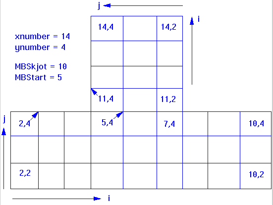
xnumber, ynumber, znumber and lnumber. There are four integers that show
the number of grid lines in the streamwise, cross-streamwise and vertical
direction. lnumber is the number of sediment sizes. This data set must be
present in the control file. The program will read these values and
allocate space for the arrays accordingly.
Vertical distribution of grid cells. This dataset must be present in the
file. A number of floats are read; equally many as grid lines in the
vertical direction. The first number is 0 and the last is 100 (%). If
there for example are 4 grid lines in the vertical direction, and the
first cell is has a height of 25 % of the depth, the second cell has a
height of 40 % of the depth and the third (top) cell has a height of 35 %
of the depth, the following data set is used:
G 3 0.0 25.0 65.0 100.0
Sediment sources. Six integers and lnumber floats are read. The integers
indicate a region of the grid. The first two are in the streamwise
direction, the following two are in the cross-stream direction and the two
last integers indicate the vertical direction. The following floats gives
the sediment concentration in volume fractions.
Example: Sediment concentration 0.001 flows into the top of the geometry n
an area given by the following cells: j=2 to j=4 and i=3 to i=5. It is
assumed that there are 11 grid lines in the vertical direction. This gives
the following data set:
G 5 3 5 2 4 11 11 0.001
Data set for calculating water surface location with an adaptive grid. Three integers and two floats:
iSurf: jSurf: kSurf:
These are three integers that indicate three grid lines. This point is a reference point, and it is not moved. In the present implementation, kSurf have to be equal to znumber + 1. If not, a warning message is sent to the boogie file, and kSurf is set to znumber + 1. The computations continue afterwards.
RelaxSurface:
This is a float that relaxes the estimation of the increment to the new recalculated water surface. Recommended values are between 0.5 and 0.95.
ConvSurface:
This float sets the limit for when the water surface should be recalculated. The water surface will be updated when the maximum residual of the equations are below this parameter. Recommended value: 0.01 - 1.0
This data set specifies water inflow on geometry sides, bed or top. Each surface is given on one G 7 dataset. It is possible to have up to 19 G 7 datasets.
On each dataset, seven integers and four floats are read. The names of these variables are:
G 7 type, side, a1, a2, b1, b2, parallel, update, discharge, Xdir, Ydir, Zdir
Each variable is explained in the following:
- type: 1: outflow, 0: inflow.
- side: 1: plane i=1
-1: plane i=xnumber,
(cross-streamwise plane)
2: plane j=1
-2: plane j=ynumber,
(streamwise plane)
3: plane k=1
-3: plane k=znumber
(horizontal plane)
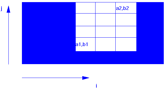
- a1,a2,b1,b2: four integers that determine the limits of the
surface. An example is shown in the figure.
- parallel: direction of the flow:
0: normal to surface
1: parallel to grid lines normal to surface
2: direction is specified (vector directions)
- update: 0 for not update, 1 for update.
(only partly implemented)
- discharge: discharge in qm/s. Note that the sign of the
discharge must correspond with the direction of the
desired flow velocity. Positive discharges indicate
discharges in positive directions.
- Xdir: direction vector in x-direction
- Ydir: direction vector in y-direction
- Zdir: direction vector in z-direction
Example: G 7 0 1 2 11 2 11 0 0 32.0 1.0 0.0 0.0
This example specifies inflow in the most upstream cross-section. The inflow area is from cell no. 2 to cell no. 11 in both cross- streamwise and vertical direction. The flow direction is normal to the cross-section. The discharge is 32 cubic meters/second.
The parameter "side" can be used to specify flux on sections that have been "amputated" by the multi-block procedure. The parameter side is then evaluated as the number of the block plus 10. Example: A geometry with one multi-block that starts at node i=30. To specify flux on wall i=29, use the G7 data set with the parameter "side" set to 11 (10+1).
Remember to define the walls of the boundary that when this dataset is used. This must be done on the W 4 data set.
Values for initial velocities. Up to 19 data G 8 data sets can be used. Six integers are read first to specify the volume that is being set. Then three floats are read, which gives the velocities in the three directions.
G 8 i1 i2 j1 j2 k1 k2 U V W
Source terms for the velocity equations. Six integers and two floats.
i1,i2,j1,j2,k1,k2, source, relax
The first six integers give the cells that are influenced by the source term. The source variable is the form factor times a diameter of a cylinder in the cell. The relaxation variable is recommended set between 1.0 and 2.0
Sediment source for multi-block border. This is used where there is inflow of sediments in a branch of a block that is cut of. An integer is first read, which tells the number of the block. Then lnumber floats are read, which is inflow of sediments for each size. This is given in kg/s. The option is not fully tested yet.
Outblocking option that is used when a region of the geometry is blocked out by a solid object. An integer is read first, which determines which sides the wall laws will be applied on. The following options are possible:
0: No wall laws are specified 1: Wall laws are used on the sides of the block 2: Wall laws are used on the sides and the top of the block 3: Wall laws are used on the sides, the top and the bottom of the block
Six integers are then read, i1,i2,j1,j2,k1,k2. These integers define the block.
Up to 19 G 13 data sets can be used.
Debug dump option, where a variable in a cell is written to the boogie file. Four integers are read. The first integer indicate which equation. Velocities in x,y and z directions are denoted 1,2 and 3, respectively. 5 and 6 are used for k and *, respectively.
The next three integers are cell indexes i,j and k.
Example: G 14 1 3 4 6 causes velocity in x-direction for cell i=3, j=4 and k=6 to be written to the boogie file for each iteration.
Up to 29 G 14 data sets can be used.
Scaling factor for mouse location in graphics routines. Default 1.0
Local vertical distribution of grid cells. This data set can be used when a different distribution of grid cells than what is given on the G 3 data set is wanted in some parts of the geometry. Four integers are read first. These tells which area are affected by the changed distribution. Then znumber floats are read, similarly to what is on the G 3 data set.
Example: G 16 2 3 1 4 0.0 50.0 75.0 100.0 when znumber is 4, gives the new distribution for the eight vertical lines i=2 to i=3 and j=1 to j=4.
Up to 20 G 16 data sets can be used.
OpenGL 3D surfaces parameters. One surface is described on each G 19 data set. Up to 50 G 19 data sets can be used.
Each data set consist of eight integers. The first integer specifies the number of the grid line. The second integer is an index showing the main direction of the grid surface. The following options are possible:
1: cross-section 2: longitudinal profile 3: plan view
The following four integer defines the corners of the surface. The last two integers are presently not used for anything, but they must be given.
Example: G 19 11 3 2 5 2 6 0 0
This gives a surface along the grid surface k=11, from i=2 to 5, and j=2 to 6.
If no G 19 data sets are given, a default data set is used this is:
G 19 1 3 2 xnumber 2 ynumber 0 0
This will give the bed of the geometry. The parameters xnumber and ynumber are given on the G 1 data set, and is the number of grid lines in the streamwise and cross-streamwise direction.
This data set is used for plotting a color graphics map where the plotted parameter is the absolute value of the velocity. The user chooses different colors and fill pattern according to the variable.
An integer is first read, which tells how many different colors and fill patterns are wanted. Then a floating point, v1, is read which marks the upper boundary for the variable. Then two integers are read. The first integer, i1, tells what color is used, and the second integer,j1, tells what fill pattern is used. All areas that have a value below v1 will be filled with the color i1 and pattern j1. Up to 20 points can be used. Example:
H 1 3 0.01 1 1 0.1 2 2 1.0 3 3
The elements which have an absolute velocity under 0.01 m/s will be filled with the color no. 1 and fill pattern 1. The elements with absolute velocity between 0.01 and 0.1 will be filled with color 2 and fill pattern 2.
The numbers of the different colors and fill patterns are given below:
No. Color 1 Green 2 Blue 3 Black 4 Cyan 5 Magenta 6 Brown 7 Red 8 Yellow 9 Pale gray 10 Dark gray 11 Dark blue 12 Dark red 13 Dark magenta 14 Dark green 15 Dark cyan 16 White
The numbers of the different density patterns are given below:
No. Patten 1 Blank 2 Density1, light 3 Density2 4 Density3 5 Density4 6 Density5 7 Density6 8 Density7 9 Density8, dark 10 Diagonal lines, SW-NE, narrow spacing 11 Diagonal lines, SW-NE, wide spacing 12 Diagonal lines, NW-SE, narrow spacing 13 Diagonal lines, NW-SE, wide spacing 14 Horizonal lines 15 Vertical lines 16 Solid
Color map plotting for water depth instead of velocity. Otherwise it is the same as the H 1 data set.
Color map plotting for sediment size instead of velocity. Otherwise it is the same as the H 1 data set.
Color map plotting for bed shear stress instead of velocity. Otherwise it is the same as the H 1 data set.
Color map plotting for turbulent kinetic energy. Otherwise it is the same as the H 1 data set.
Color map plotting for sediment concentration. Otherwise as H 1.
Color map plotting for bed level changes. Otherwise as H 1.
Specification of isoline values for ContourMap plot. First, an integer is read, which gives the number of isolines. Then, this number of floats are read. The floats specify the isolines. Example:L 6 55.0 56.0 57.0 58.0 59.0 60.0If the geometry has bed levels between 55 and 60 meters, and the user chooses bed levels from the graphics options, a contour map of the bed levels will be displayed. There will be contour lines for each meter, from 55 to 60 meters.Default: The program finds the maximum and minimum value of the variable in the field, and uses 5 lines located between the values.If more than 5 lines are displayed, all lines will be black. Otherwise each line will have different color.Note that sometimes there may be errors in the contouring, if the contour line and the value are identical. This can often be the case for plotting bed levels. To avvoid this problem, add a very small value to the values on the L data set. For example, if the above data set is used and there is a problem for the 57.0 contour line because the bed level at one of the grid intersections are 57.0, change the data set to:L 6 55.0 56.0 57.0001 58.0 59.9 60.0
P 2
Five floating points that give scaling for the graphical presentation. The first three gives scales in streamwise, cross-streamwise and vertical direction. The fourth and fifth give movements in left-right and vertical direction. Defaults: 1.0 for the scales, and 0.0 for the movements.
P 3
Four integers that give initial location of the graphical plots in streamwise, cross-streamwise and vertical direction, and sediment fraction number.
P 4
A character that indicates initial type of plot. "g" gives the grid, "v" gives velocity lines, "V" gives velocity vectors, "c" gives concentration.
W 1
Manning's number, discharge and downstream waterlevel. This dataset must be present in the file. The parameters given here are used to generate the waterlevel for the calculations using a standard backwater calculation.
W 2
Water surface initialization array of integers. The first integer tells how many numbers there are in the array. The next numbers tell which cross- sections are going to be used in the initialization of the water surface of the grid. The integers must be given in rising order, and start with 1. This dataset must be present in the file.
W 3
Specification of multiple blocks for the multi-block water flow module. First an integer that indicates the number of extra blocks is given. The maximum value is 9. Then two integers for each extra block are given. The first integer tells where the block is cut off. The second integer tells where the block is added. If the second integer is negative, the block is added on the left side of the main block. Otherwise it is added on the right side of the block. This is explained with an example on the figure below. The corresponding dataset would be: W 3 1 10 -5
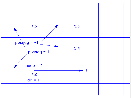
W 4
Specification of extra walls for the multi-block water flow module. Seven integers have to be given for each wall. There can be up to 29 walls, and each wall is described on one W 4 data set.The variable names are:W 4 dir,posneg,node,a1,a2,b1,b2The first integer, dir, indicates the plane. 1 is the j-k plane (cross-section), 2 is the i-k plane (longitudinal section) and 3 is the i-j plane (seen from above).The second integer, posneg, indicates if the wall is in the positive or negative direction of the node. The coordinates are given for nodes. 1 or -1 is given. If 0 is given, a previously set wall is deleted.The third integer is the number of the node plane.An example is given in the figure below. The figure shows the i-j plane. The wall is to be given on node i=4. If the second integer, posneg, is 1, then wall laws are applied on the wall upstream of node 4, in the negative i-direction. If posneg = -1, then the wall laws are applied on node 4 if the cell in the downstream i-direction (line i=3) is a wall.
The four following integers are indexes a1,a2,b1,b2, which gives the two-dimensional coordinates for the corner points of the part of the plane that is described. The four integers are the same as given on the G 7 data set.
W 5
Different Manning's values than the default value for cross-sections. An integer is first read, which tells how many cross-sections are read. Then an integer and a float is read for each cross-section. The integer tells which cross-section is changed, and the float tells the Manning's value. Several W 5 data sets can be used.
W 6
NoMovePoint - a point which is used in the GridEditor. Two integers are read, which is the numbers of the i and j grid lines. The intersection of these lines are not moved by the elliptic grid generator. One W 6 data set is required for each NoMovePoint. Maximum 199 points can be used.The W 6 data set is usually generated by the Grid Editor.
W 7
Attraction point used in the GridEditor. Each W 7 data set represents attraction to one grid line or point. Maximum 199 attraction points can be used. An integer is read first which tells the type of attraction. The following options are given:0: Point attraction in i-direction 1: Point attraction in j-direction 2: Line attraction in i-direction 3: Line attraction in j-directionThen two integers are read, which tells which grid line intersection the attraction is towards. For the line attraction, only one of the integers are used. Then the two attraction parameters are read, which are floats.The W 7 data set is normally generated by the Grid Editor.
S
Integer that gives the number of the sediment fraction, float that gives the size of the sediments for these fraction, float that gives the fall velocity for the fraction.There must be lnumber datasets like this in the file, as long as sediment concentration is to be calculated. All numbers are given in SI units, that is, the grain size is given in meters and the fall velocity is given in meters/second. This data set must be present when sediment transport is calculated.This dataset defines the grain sizes that are used in the program. Note that this applies for both the grain sizes in the bed and in the suspended sediment calculation. The grain sizes should be numbered from 1 to lnumber, where size 1 is the coarsest size, and the following sizes have decreasingly smaller diameter.
N
These data sets define different grain size distributions for the sediments that are in the bed when the calculation starts.Maximum 10 different samples can be used.Each sample has its own number. This starts with zero, and increases sequentially to the total number of samples minus one.First, an integer for the number of the sample is given. The second integer shows which size is described. The third number is a float, which gives the fraction of the size in the sample. It is required to have lnumber N data sets for each sample. These data sets must be present when sediment transport is calculated.The number of N datasets that is required is:(number of grain size distributions) x (number of sediment sizes)Note that if only deposition is calculated, it is not necessary to specify the N data sets. However, if the data sets are specified, the program will control that the sum of the fractions are unity.
B
This data set gives where the samples (from the N - data sets) are placed in the geometry before the calculation starts.The first integer indicates the number of the sample. The four following integers give the number of the corner cells on a rectangle of the bed. The sample is placed on the bed from i=second integer to i= third integer and j=fourth integer to j=fifth integer. A B data set overwrite previous B datasets.The dataset B 0 0 0 0 0 tells that sample no. 0 covers the whole bed.
I
Inflowing sediments. First integer shows which sediment fraction is simulated. Second number is a float that is the amount of inflowing sediment of this size in kg/s. lnumber of these data sets must be present when sediment concentrations are calculated. Note that the I dataset follows the sizes on the S data set, but it has nothing to do with the N and B data sets.
K 1
Number of iterations for flow procedure and number that determines the minimum iterations between updates of water surface. Two integers. Default: K 1 40000 50000
K 2
Two integers that indicate if laws of the wall are being used. The first integer applies to the side walls. The second integer applies for the surface. 0 is used for wall laws, and 1 for free surface. Wall laws are always used for the bed, if not changed by the W 4 data set. Default: 0 1.
K 3
Relaxation factors. Six floats. For the three velocity equations, the pressure correction equation and the k and * equation.Default: K 3 0.8 0.8 0.8 0.2 0.5 0.5
K 4
Number of iteration for each equation. Six integers.Default: K 4 1 1 1 5 1 1
K 5
Block-correction index for each equation. Six integers. If 0, no block- correction. If 1, the block-correction is used.Default: K 5 0 0 0 0 0 0 Note that the block-correction may not work with the SOU scheme.
K 6
Six integers are read which determines whether the SOU or POW scheme is used. If 0 POW is used, if 1, SOU is used. Note that presently the multi- block flow module may not converge completely when the SOU scheme is used with multiple blocks. This may be due to a bug. SOU will work if there is only one block.Note that the flow module will always use the POW scheme for the pressure-correction equation.Default: K 6 0 0 0 0 0 0
K 9
A character deciding whether SIMPLE or SIMPLEC is used. Y= SIMPLE, N = SIMPLEC. Default: Y
K 10
A character that decides which solver is used. Y = Gauss-Seidel solver, N = TDMA solver. Default: Y
The boogie file
This is a file that shows a print-out of intermediate results from the calculations. It also shows parameters as average water velocity, shear stress and water depth in the initialization. Trap efficiency and sediment grain size distribution is also written here. If errors occur, an explanation is also often written to this file before the program stops. The file contains the data that is normally written to the screen in a DOS program.The option D on the F 1 data set will give additional print-out to the file.Initially in the file it is written how much memory that is occupied by the arrays that are dynamically allocated. To estimate the total recommended memory requirement for SSIIM, add 1 MB to this value.A table then follows, which shows the cross-sectional area, hydraulic radius, average velocity and water level at the cross-sections that have been used for initializing the water surface. If the option D on the F 1 data set is used, this information is written for all the cross-sections additionally. Then a table of waterlevels for all cross-sections follows:Loop1,iter,area,radius,velocity,waterlevel: 12 1.002389e+00 1.002389e+00 9.976163e-01 1.002390e+00 Loop1,iter,area,radius,velocity,waterlevel: 11 1.001588e+00 1.001588e+00 9.984146e-01 1.001589e+00 Waterlevel = 1.000398 meters for cross-section i = 10 Waterlevel = 1.000797 meters for cross-section i = 9 Waterlevel = 1.001195 meters for cross-section i = 8If SSIIM terminates and the boogie file contains the following message: Error, negative areas for cell i=13, j=2, or some other combinations of i and j, then there is an error in the koordina file. The indexes denote the cell number, so for i=13, j=2, the x and y coordinates for the following grid line intersections should be checked: (13,2); (13,1); (12,2) amd (12,1).If the MB-flow module is used, the residual norms are written. Then follows a sequence of two lines for each iteration of MB-flow. An example with four iterations is shown below:Iter: 5, Resid: 1.69e-05 4.10e-06 2.73e-05 1.17e-04 1.38e-02 1.13e-02 Cont: 9.23e-08, DefMax: 1.65e-03, U,V,W(96,7,20): 6.40e-01 -5.14e-03 5.76e-02 Iter: 6, Resid: 1.62e-05 3.85e-06 2.62e-05 1.10e-04 1.31e-02 1.08e-02 Cont: 9.23e-08, DefMax: 1.56e-03, U,V,W(96,7,20): 6.40e-01 -5.14e-03 5.76e-02 Iter: 7, Resid: 1.57e-05 3.65e-06 2.50e-05 1.04e-04 1.25e-02 1.03e-02 Cont: 9.23e-08, DefMax: 1.48e-03, U,V,W(96,7,20): 6.40e-01 -5.14e-03 5.76e-02 Iter: 8, Resid: 1.51e-05 3.46e-06 2.38e-05 9.86e-05 1.18e-02 9.77e-03 Cont: 9.23e-08, DefMax: 1.41e-03, U,V,W(96,7,20): 6.40e-01 -5.14e-03 5.76e-02The first line has the word "Iter" at first. Then an integer follows, which shows the number of the iteration. In the example above this runs from iteration number 5 to 9. Then the residuals for the six equations are shown. The x,y and z velocity equations are first, then the pressure equation and the k and epsilon equation follow. All these must be under 0.001 before the solution has converged.The second line starts with the word "Cont". Then a floating point value is shown. This is the sum of all the water inflow and outflow in the geometry. This should be a very low value, typically under 10E-7. If a larger value is given, check the boundary conditions. Then the word "DefMax" is written. The residual for the cell with largest water continuity defect is then written. The indexes for this cell are then written, with the velocities in the three directions for this cell. In iteration 9 for the example above, the maximum water continuity defect was 1.41e-3 kg/s for cell i=96, j=7, k=20. The velocity in the x-direction for this cell was 0.64 m/s, the velocity in the y direction was -5.14 mm/s and the velocity in the vertical direction was 5.76 cm/s.If 3D changes in the water surface elevation is calculated, the water surface elevations along the centerlines in the two horizontal directions are written to the boogie file. This is done for each update. An example of some of these results is shown below:WL(20,1) = 1.012947e+00 WL(20,2) = 1.012427e+00 WL(20,3) = 1.011113e+00 WL(20,4) = 1.009520e+00 WL(20,5) = 1.007900e+00If the sedimentation calculation is used, the fluxes through the four side walls and the trapped sediments are written for each size. This is written for each 100th iteration. An example is shown below:Trap efficiency after 24700 iter: all values in kg/s l=1: Trapped: 230.015, Fluxes (I1,I2,J1,J2): 229.843, 2.95575e-20, 0, 0 Resid: 0.000750 l=2: Trapped: 485.265, Fluxes (I1,I2,J1,J2): 499.657, 85.56, 0, 0 Resid: 0.142433 l=3: Trapped: -2617.23, Fluxes (I1,I2,J1,J2): 269.815, 3489.59, 0, 0 Resid: 2.233171Three sizes are given in the example. For size 2 the inflow is 499.657 kg/s, the outflow is 85.56 kg/s and 485.256 kg is trapped. The residual is the continuity defect divided by the inflow. The convergence criteria is given on the F 4 data set. The solution is converged when the average residual is under the convergence criteria.After the sedimentation calculation has finished, the time step is written. A further explanation of the time step is given in [4].If the bed changes are calculated this is also written to the file. The bed changes are given in meters. An example is given below:BedMove(10,8) = 1.009495e-03 meters BedMove(10,9) = 1.030140e-03 meters BedMove(10,10) = 1.019934e-03 metersIn the example, the deposition in cell i=10, j=10 causes the bed to rise 1.02 mm during the given time step.For the transient sediment calculation routine, sediment continuity is written for each time step. All numbers are in cubic meters.Sedim. continuity: In, Out, DcDt, Bed, Move, ContDef., MoveDef: Dt: 0.453509 20.995623 -20.666748 0.355497 0.110065 0.230863 0.245432 Sum: 0.888430 50.468110 16.613033 - 66.460044 -68.192414 -0.267331 1.732371The first line gives the names of the variables in the two lines below. The second lines give data for each time step, while the third line gives data for accumulated time.The first number is the inflow of sediments. The second is the outflow of sediments. The third is the accumulated sediments in the water body. The fourth is the calculated bed changes. The fifth is the actual bed changes. The sixth is the continuity defect, and the second is the defect because of the bed changes. The last two numbers should be small compared with the total flux in the geometry.
The koordina and koomin files
The koordina file describes the bed of the geometry. An example is show in the figure below. The grid can be made using a map, a spreadsheet or the Grid Editor
Grid with numbering of lines and cells
The necessary input data is the x,y and z coordinates of the points where the grid lines meet. The format of the data is given below.i j x y z An example 1 1 0.34 0.54 0.11 1 2 0.35 0.66 0.12The first two numbers are integers, while the following three are floats. The numbers are read in a free format, which means that the distance between them does not matter. The sequence of the points are not important, as long as all points are included. This is not controlled by the model, so the user must do this by looking at the grid in the graphic modules of the program.If a tunnel is simulated, or the user wants to specify the water surface, an additional floating point number is read for each line. This gives the top level for each grid intersection. An example:1 1 0.34 0.54 0.11 1.21 1 2 0.35 0.66 0.12 1.33To make SSIIM read the last float, the K 1 data set in the control file must be: K 1 0 0Some words about indexing and numbering of grid lines and cells. The variable names for the number of grid lines in the three directions are:xnumber : number of cross-sections ynumber : number of longitudinal lines znumber : number of horizontal linesThe numbering of the grid lines goes from 1 to xnumber in the streamwise direction, and similarly for the other two directions.However, the grid lines define cells between the grid lines. The variables are calculated in the center of each cell. This means that a numbering for cells also is required. The word node is often used for the center of a cell.From a geometrical view of the grid, it is observed that the number of lines always exceeds the number of cells by one in each direction. When the arrays are defined, it is therefore a choice for the programmer to start the numbering of the cells on one or two. The choice that is made in this program is that the numbering starts on two. This means that the cell that is defined by grid lines i=1 and i=2 and j=1 and j=2 has the number (2,2). Cell number (1,1) does not exist. The numbering of the cells is also shown in Fig. 1. The numbering of the grid lines is shown with the <,> sign, while the numbering of the calculation nodes is shown with the (,) sign. The grid is non-staggered.If SSIIM terminates and the boogie file contains the following message: Error, negative areas for cell i=13, j=2, or some other combinations of i and j, then there is an error in the koordina file. The indexes denote the cell number, so for i=13, j=2, the x and y coordinates for the following grid line intersections should be checked: (13,2); (13,1); (12,2) and (12,1).The data on the koordina file defines a surface. It is possible to make a file with exactly the same format and call it koomin. This surface is then used as a minimum elevation surface for bed changes. The bed will not be lowered under this surface.
The geodata file
This file contains a number of x,y and z coordinates. An example is shown below:E 2.2 3.3 3.4 E 4.5 3.3 2.2 E 3.3 4.2 1.2The purpose of this file is to use geometrical data that has been obtained from the field, a digitized map or a GIS system. These data would normally not fit into a grid like the koordina file.The file is used in three modules in the program. The first module is the GridEditor, which can display the points in the file with the grid. This makes it easier to generate the grid. The Utility option of the menu and the Show geometrical points option in the pull- down menu activates this. The grid points are displayed with different colors according to which level they are.The second use for this file is also in the GridEditor. It is then used in the Make bed interpolations for generating the z values for the bed of the grid. A linear interpolation procedure is used.The third use is to make the Porosity file. The module that does this is activated from the main menu of the user interface, from File and Make porosity file in the pull-down menu.
The bedrough file
This file is used to give a roughness height to individual bed cells. Values in this file overrides the value calculated from Manning's coefficient, and the value given on the F 16 data set. On each line a character, two integer and a float are given. The first character is a B, and the two following integers are indexes for the bed cell. The float is the roughness in meters. An example is given below:B 19 2 0.001 B 19 3 0.001 B 19 4 0.001
The porosity file
Note: When using the porosity file, use a P on the F 7 data set.This file is used when the bed of the river is covered by stones, and a porosity term is used in some of the cells. This file describes the location and magnitude of the porosity in the geometry. An example is given below:P 17 6 3.349774 3.399189 3.450101 3.499517 0.000000 0.700000 0.833333 1.000000 P 17 7 3.358273 3.413603 3.470610 3.525940 0.000000 0.653846 0.807692 1.000000 P 17 8 3.403323 3.426084 3.449536 3.472297 0.000000 0.642857 0.785714 1.000000First, the character P is read. Then two indexes for the i and j number of the bed cell is read. Then four vertical levels are read, which have the same zero reference as the koordina file. The porosities in each of these levels are then read.The porosity file can be made from a koordina file and a geodata file. The module that does this is activated from the main menu of the user interface, from File and Make porosity file in the pull-down menu. The procedure goes through each element and used the points in the geodata file to obtain the data.
The innflow file
This file is used to read velocities in three directions for the upstream boundary condition. The program searches for this file, and uses the data on the file if it exists. If the file does not exist, a warning message is written to the boogie file, and the program proceeds normally.On each line the velocities in a cell of the upstream cross-section are given. First, the character E is written. Then the indexes j and k (horizontal and vertical) are given. Then the velocity components in the x,y and z directions are given. An example is given below:E 2 2 0.299115 0.023009 0 E 2 3 1.79469 0.138055 0 E 2 4 1.9941 0.153394 0 E 2 5 2.19351 0.168733 0The file does not have to contain values for all the nodes. The normal initialization procedures are applied first, and then the innflow file is read. The nodes that are not present in the innflow file will keep the values from before the file was read.
The loggfil file
This is a file that is used to log bed changes between each time the bed is changed. The bed changes are written with the "append" mode in C, so that for the file to be updated, it must exist before SSIIM writes to it. What is written to the file will be appended to what is present in the file.What is written to the file is a time step for each change, together with the bed changes for each cell in meters. The bed sediment grain size distribution for each time step is also written to this file.When SSIIM starts, it looks for a file called loggfil.pre, and if it exist, it uses this file to change the bed and give initial bed sediment grain size distribution. If one decides to start from a previous time step, one must have copied loggfil to loggfil.pre before starting SSIIM.loggfil is written from the Bedchange+ option in the Map graphics module.The loggfil file is never overwritten by the program. New bed changes are appended to the end of the file. The user must therefore take care so that only the relevant data exist in the loggfil and loggfil.pre files.Note that if the program does not find the loggfil.pre file, a warning is written to the boogie file, and the program proceeds normally.
The result file
This file contains the results from the water flow calculations. The file is written when the prescribed number of iterations have been calculated or when the solution has converged. The results are velocities in three dimensions, k, *, pressure, and the fluxes on all the walls of the cells. The data from this file is used as input for the sediment flow calculations. This file can also be read when the user wants to start the water flow calculations from where the result file was last written (hot start).An example of a result file:Results from SSIIM - flow, iter = 12910 Residuals: 0.000732 0.000588 0.000002 0.000003 0.001000 0.000000 Roughness : 0.050000 C 54 9 11 i j k u v w k e f1 f2 f3 p D 1 1 1 0.00000000e+00 0.00000000e+00 0.00000000e+00 0.00000000e+00 0.00000000e+00 0.00000000e+00 0.00000000e+00 0.00000000e+00 0.00000000e+00 D 1 1 2 0.00000000e+00 0.00000000e+00 0.00000000e+00 0.00000000e+00 0.00000000e+00 0.00000000e+00 0.00000000e+00 0.00000000e+00 0.00000000e+00 D 1 1 3 0.00000000e+00 0.00000000e+00 0.00000000e+00 0.00000000e+00 0.00000000e+00 0.00000000e+00 0.00000000e+00 0.00000000e+00 0.00000000e+00 D 2 4 7 6.31143968e-01 2.02894592e-01 -6.80367016e-05 6.47305125e-03 3.85539263e-04 3.47858729e+03 -5.19507052e+02 1.39776552e+03 1.91355310e+02 D 2 4 8 6.38189711e-01 2.05198514e-01 -2.09522025e-04 6.40727451e-03 3.13804122e-04 3.54203761e+03 -5.25291012e+02 1.09548199e+03 1.91350056e+02 D 2 4 9 6.42687814e-01 2.06670571e-01 -3.70305526e-04 6.37079494e-03 2.71714390e-04 3.58421958e+03 -5.28978103e+02 7.51732364e+02 1.91343817e+02The first lines gives the residuals, the roughness and the grid size. Then each line gives the nine values for one cell. The letter D starts the line, then the three indexes for the cell. Then the three velocities, the k and epsilon values. Then the fluxes in the three directions and finally the pressure. All the parameters are placed on one line in the file.All the results are given in SI units, so that for example the velocities are in meters/second and the pressure is in Pascal, or Newton/m2.
The conres file
This file is written after the sediment concentration calculation has finished. Each line in the file contains first three indexes indicating for the node number. Then the total concentration is written and then lnumber floats that give the concentration for the sizes. An example is given below:1 1 21 0.000000e+00 0.000000e+00 0.000000e+00 0.000000e+00 0.000000e+00 1 2 2 5.075079e-04 0.000000e+00 1.026459e-04 1.030081e-04 1.032351e-04 1 2 3 4.064470e-04 0.000000e+00 1.011788e-04 1.015358e-04 1.017596e-04 1 2 4 4.004061e-04 0.000000e+00 9.967497e-05 1.000267e-04 1.002471e-04If a file conres.pre exist, this will be read by the program before the sediment calculation starts. The conres.pre file has the same format as the conres file.
The interpol and interres files
Vertical profiles of velocity or concentration are sometimes needed. Coordinates for the locations where the profiles are wanted are given in this file. When the write results routine is activated and the integer on the F 48 data set in the control file is above 1, it will search for this file. If this file is not found, it will proceed normally and write the result or the conres file. If the interpol file is found and the integer on the F 48 data set is above 1, the program will not write to the result file, but write the interpolated vertical velocities to a file named interres. An example of an interpol file is given below:M 2.03 0.5 M 4.06 0.39 M 4.06 0.5The character M is read first, and then the x and y coordinates for the point one wishes to interpolate the vertical profile to. If the value on the F 48 data set is 3 the concentrations are interpolated. If the value on the F 48 data set is 2, the velocities, k and * are written to the file. If the value on the F 48 data set is 1, the bed levels are written (no profile, only one point). The results are written to a file called interres.An example of an interres file is given below:C 9.250000 0.100000, size = 0 1.530130 0.000000e+00 1.491877 5.266262e-05 1.415370 9.303652e-05 1.338864 1.349549e-04 1.262357 1.740915e-04 1.185851 2.075269e-04The first line starts with a C, and then the x and y coordinates of the vertical profile is given. Two columns follow. The first column is the z value of the vertical profile. The second column is the concentration. If velocities are interpolated instead of concentrations, an M is written on the first line instead of the C. Instead of the concentration column, five calamus are written. The variables in the columns are: velocity in x,y and z directions, k and epsilon.Note that the procedure for writing the interres file changed from SSIIM version 1.3 to version 1.4.
The verify file
This file is used as input for the VerifyProfile graphics option. The user can present calculated velocity or concentration profiles together with measured values. Up to 20 vertical profiles in a section of the geometry can be shown. The horizontal location of the profiles are determined by the user, so this method of presentation can be used for both cross-sections, longitudinal section or other user-defined sections. An example of a verify file is shown below:P 40.0 10.0 3 5.0 0.5 0.1 6.5 0.6 0.12 7.0 0.8 0.05 P 70.0 10.0 2 6.0 1.0 0.1 8.0 1.5 0.8Each profile is identified with a capital P. Then the x and y coordinates of the point follow. The coordinates are given in the same system as the grid, or the koordina file. After the coordinates, an integer is read. The integer tells how many points are measured in this profile. Up to 11 points can be given. On the following lines the data is given. There must be the same number of lines as the integer on the P line. Three floats are given on each line. The first is the vertical coordinate where the data is taken. This is given in the same coordinate system as the grid, or the koordina file. The following two floats are velocities or concentrations, depending on what is calculated. If velocities are calculated, the second float is the velocity component in the x-direction and the third float is the velocity in the y-direction. If concentration is calculated, the second float is the measured concentration and the third float is a dummy number which is not used. If concentrations are given, the user can choose in the graphics presentation wheter a total concentration or a fractional concentration is presented.The example above gives two profiles. The first is located at x = 40.0 meters and y = 10.0 meters. Three data points have been measured. The first point is located at global coordinate z = 5.0 meters, and have a measured x-component velocity of 0.5 m/s and a y- component velocify of 0.1 m/s. The second point is located at global coordinate z = 6.5 meters, and have a measured x-component velocity of 0.6 m/s and a y-component velocity value of 0.12 m/s.Note that this file changed from SSIIM version 1.3 to version 1.4.
The timei and timeo files
There are two files that are relevant to time series calculations. The first file, timei, is an input file for time series of discharge, waterlevel, sediment concentration and control for output. The second file, timeo, is an output file with time series from the model.The timei file reads two types of data sets. The first type controls the output to the timeo file. This data set begins with a capital O, and then reads a float, Time, and an integer, Vars. Time is the time for when the print out starts, and Vars tells how many variables are written to the timeo file for each time step. Maximum 25 variables can be written. A maximum of 20 control output data sets can be used.After reading Time and Vars, the next lines read which variables are printed and in which cell. Vars lines are read. Each line starts with a lowercase character, and then three integers (four in case of sediment concentration) are read. The integers indicate which cell the variable is located in. If sediment concentration is read, the last integer tells which fraction is written. 0 indicates the sum of the fractions. The characters corresponding to different variables are listed below:character: variable: u velocity in x-direction v velocity in y-direction w vertical velocity p pressure k turb. kin. energy e epsilon d turb. diffusion z vertical grid elevation c concentrationThe second type of data set is input data. The line starts with a capital I, and then five floats are read. The first float indicates the time for when the following variables are used. The second float is the upstream water discharge. The third float is the downstream water discharge. The fourth float is the upstream water level, and the fifth float is the downstream water level. Sometimes one of the last variables are unknown, and then a negative value can be inserted and the program will try to calculate the value.If the TFS method is used, lnumber floats are read additionally, indicating the upstream inflowing sediment transport.An example of a timei file is given below:O 0.0 6 u 2 2 2 c 2 2 2 0 p 2 2 2 z 41 3 6 z 1 2 1 z 2 2 1 I 0.0 10.0 10.0 -20.0 19.5.0 0.000 I 100.0 10.0 10.0 -20.0 19.0 0.000 I 200.0 10.0 10.0 -20.0 18.5 0.000 I 300.0 10.0 10.0 -20.0 18.0 0.000 I 400.0 10.0 10.0 -20.0 17.5 0.000The timeo file gives the output time series from the calculation. For each time step, a line of variables are written to the file. Each line has Vars floats, according to which variables were given in the timei file. In the above file six variables are written. The first variable is the velocity in x-direction for cell (2,2,2). The second variable is the sum of all sizes of concentration for cell (2,2,2). The pressure and vertical grid elevations for various grid intersections are written.The second group of parameters in the timei file is an input time series. Each time step in the series are given on one line. The line starts with a capital I. Then the time step is given. Then four floats are read. This is the upstream and downstream water discharge and upstream and downstream water level, respectively. If a negative value is given, the program will try to calculate the value. The last float(s) are sediment concentration(s) for the various sediment sizes. These are only read if the transient sediment calculation is used. Note that the time steps does not have to correspond to the time steps of the program. The sum of the calculated time steps is calculated by the program and compared with the time step in the file. If the calculated time exceeds the time from the file, the values from this data line will be used. The times must be in increasing order.An example of a timeo file corresponding to the above timei file is given below:0.0000e+00 2.0000e+00 8.804354e-01 6.837692e-04 -1.853305e+01 1.950000e+01 1.792479e+01 4.0000e+00 9.185002e-01 7.081983e-04 -3.949717e+01 1.950000e+01 1.792458e+01 6.0000e+00 1.100297e+00 1.121773e-03 5.289925e+01 1.950000e+01 1.792421e+01 8.0000e+00 1.156041e+00 1.389383e-03 8.122703e+01 1.950000e+01 1.792374e+01 1.0000e+01 1.207883e+00 1.614782e-03 9.418469e+01 1.950000e+01 1.792317e+01Each line corresponds to a time step. A time step of 2 seconds have been used. The first float is the calculated time. The second float is the velocity in cell (2,2,2). Then the sum of the concentrations in cell (2,2,2) is written. Then the pressure and the vertical grid elevations.This format is chosen so that it is easy to import the file to a spreadsheet for presentation.
The forcelog file
This file contains time series of the forces on one or more obstacles for the transient free surface calculation. One line is written for each time step. An example of a forcelog file is shown below:Forces on block 1 : 271.062, 0.099838 N in x and y direction Forces on block 1 : 398.574, 0.082644 N in x and y direction
The xcyc and koosurf files
The two files xcyc and koosurf contain the geometry of the grid. This is used when restarting calculations which have changed the grid.The koosurf file is identical to the koordina file, except that the surface level is also written for each line. This is similar to using the koordina file with the tunnel option.The xcyc file contains the x, y and z values of all the grid intersections.When writing the files from the menu, both files will be written. When reading the files, SSIIM will try to read both files, but if the xcyc file is missing, it will only read the koosurf file. The internal grid nodes will be generated by linear interpolation, as given on the G 3 data set in the control file.If the internal nodes of the grid are generated by linear interpolation, the only necessary file is the koordina file. However, for calculations where some part of the grid moves, and some is outblocked and does not move, it is necessary to save the xcyc file, and let SSIIM read this.
Advice for users
Advice for new users
Generally, it is advisable to start with reading this manual. It is important to understand that the model is made up of several sub-models. This is reflected in the different choices in the main menu which is used to start the sub-models. Some models can be run simultaneously.The hardware requirements for running the program are mainly focused on having enough RAM. In the beginning of the boogie file it is printed how much RAM the program allocates for the arrays. This can be added to the RAM requirement for the program itself, about 1 MB, plus what the operating system requires. An estimate for the amount of RAM is thereby obtained. OS/2 will use the harddisk as extra memory if there are not sufficient RAM. The penalty is that the program runs very much slower. This situation can be detected by observing if the system swaps to the harddisk while running only the SSIIM program. The water flow module may take from some hours to some days to converge for a typical case, when there is enough RAM. However, under OS/2 it is not any problem to let the program run in the background while doing other tasks on the computer.An advice for the first-time user is to run the tutorial and one of the example cases. Try to modify some of the parameters and run it again. Often the user wants to simulate a particular case. It is then advisable to try to find a similar example case and modify this step by step.Some words about crashing the program and input control. There are various controls for input and checking of intermediate results. If any of these controls finds something wrong, an error message is written to the boogie file, and the program may terminate. Therefore, if the program suddenly stops, and the main user interface disappears, check the boogie file for possible error messages.Two files are required to run the program. These are called koordina and control. The koordina file contain the grid. The control file contain the rest of the necessary parameters. The newer versions have new options for making the input data for the control file, and there is also a Grid Editor that can be used to make the koordina file.Finally, the results from the program ought to interpreted according to:- Possibilities of bugs in the program making errors - Previous cases where the results have been compared with measurements - Numerical errors, like false diffusion, grid independence, etc. - Accuracy of boundary conditionsKnowledge and experience in computational fluid dynamics and hydraulic engineering are essential for the assessment of the validity and accuracy of the results. Also see advice for interpretation of results.
The grid
Making the grid is often the most time-consuming process in the preparation of input data for SSIIM. The general idea is to divide the water body into cells. The size and alignment of the cells will strongly influence the accuracy of the calculation, the convergence and the computational time.The grid used in SSIIM is structured. This can make it difficult to adapt the grid to complex geometries without loss of accuracy or slow convergence. In the following there are given some guidelines of how to make a good grid. Also, it is recommended to read Chapter 4.4 first, to understand the index system of the grid lines.If the water body is rectangular, it is possible to use a spreadsheet to make the grid. However, in most cases, the fastest way to make the grid is to use the GridEditor. It is recommended to read Chapter 3.3 and try the tutorials to get to know the GridEditor.When the grid is made, a backwater calculation is carried out to determine the initial water surface. The water surface will therefore have a downward slope from cross-section j=1 to cross-section j=ynumber. The parameter ynumber is the number of cross-sections. Also, by default, the given discharge is flowing into cross-section j=1 and out of cross- section j=ynumber. Therefore, when making the grid, be sure that the line j=1 is the upstream cross-section of the geometry, where most of the water enter the geometry.Here are some advice on how to shape the cells.1 Make the grid line intersections as perpendicular as possible. It is not adviceable to have intersections with an angle of less than 45 degrees. Non-orthogonality in the grid will make the convergence slower. It is recommended to use the elliptic grid generator to make the grid smoother.2 Try to align the grid lines in the streamwise direction paralell to the velocity vectors. This will decrease false diffusion.3 The distortion ratio should not be too great. The distortion ratio is the dimension of the grid in one direction divided by the dimension in another direction. Some people say this should be less than 2 (two), but other people have obtained good results for ratios up to 10. On occations, ratios of up to 100 have been used. This gave reasonable results, but it required very low relaxation coefficients and an extremely large number of iterations to converge.4 The size of a grid cell should not be too much larger than its neigbours. Some people say the increase in size should not be greater than 20 %. On some occations this value have been over 1000 % (a factor 10). Some of these cases gave reasonable results, but other cases gave unphysical results. A recommendation is to try to stay within 50 %, but if much larger values are used, be aware that unphysical results may occur. Unphysical results can be velocity vectors that point in another direction than what seems natural, for example not paralell to walls.The following two chapters give more advice on convergence and interpretation of the results:Experience with convergence for the water flow calculationAdvice for interpretation of results
Experience with convergence and crashes
There are three ways SSIIM can crash:1. The program stops calculation and the dialog box says there is an error.2. The program stops and exits, the menu and the dialog box disappear.3. The program stops with an OS/2 system error, usually floating point invalid operation, overflow or underflow error.Often an error message is written to the boogie file before the crash occur. This happens particularly for type 1 and 2 of this list above. If an error in the input files are detected, an error message is written to the boogie file and type 2 crash occurs. If the program crashes, it is therefore recommended to take a look at the boogie file. If crash type 1 occurs, it is also possible to look at the graphics to try to see where in the geometry the problem is.If the boogie file contains the following message: Error, negative areas for cell i=13, j=2, or some other combinations of i and j, then there is an error in the koordina file. The indexes denote the cell number, so for i=13, j=2, the x and y coordinates for the following grid line intersections should be checked: (13,2); (13,1); (12,2) amd (12,1).Crashes during initiation of the water surface
The initial water surface calculation is a 1 D backwater calculation using Manning's formula for the friction loss. When this does not converge the program may crashes with no error messages, except an OS/2 error message that tells that the program had caused a floating point overflow error. This usually happens when there is supercritical flow somewhere in the geometry. The remedy is twofold:
1. Increase the number of cross-sections for the initiation on the W 2 data set in the control file.2. Choose higher Manning's friction factors on the W 1 or the W 5 data set in the control file.This procedure has so far worked for all the cases where this problem has occurred.Crashes with underflow error
For some cases the program can crash with an underflow error (type 3 crash). This happens particularly when some part of the geometry is blocked out. The reason is that a variable is multiplied with 10e-30 for each outblocked cell, and when the solver multiplies these together and there are sufficient outblocked cells to get below 10e-300 an underflow exception occurs. To prevent this there has to be an if-statement inside the solver loop, and this slows down execution of the program slightly. Therfore two solvers are incorporated, and if the F 43 data set is used, the solver with control of underflow error is used. Calculations with default values of F 43 will not check for underflow errors.
Convergence
There are three main calculation algorithms in SSIIM:
1. Initial water surface calculation 2. 3D water flow field 3. 3D sediment flow fieldThe sediment calculation has always converged, although sometimes it may take some time. The main problem is then to get the 3D water flow field calculation to converge. Generally, in computational fluid mechanics cases it is often a problem to get the solution to converge. Two factors are important:- A good grid. - Proper relaxation coefficients.It is presumed that the boundary conditions are correct, which is always a good thing to check in case of low convergence or strange results.Experience shows that the degree of non-orthogonality of the grid will affect the convergence. A higher degree of non-orthogonality will give slower convergence. A slower convergence will also be experienced where strong gradients are present. This applies for example at the inflow of a jet from a wall.For the convergence of the k and epsilon equations for river problems, the size of the cell closest to the bed is important. This can be changed by changing the second number in the G 3 data set in the control file. This parameter also depends on the roughness of the bed. The size of the bed cell should increase with increasing roughness. The height of the bed cell should not bee too much smaller than the roughness of the bed.The default values of the relaxation coefficients are set to 0.8 for the velocity equations and 0.2 for the pressure-correction equation. For k and epsilon, 0.5 is used as default. The values of the relaxation coefficients for the velocity equations and the pressure-correction equations are presumed to give an optimum convergence for the average flow case. Values of 0.5 for all equations will often give a slower convergence, but with less probability of divergence. Theoretically, the sum of the relaxation coefficient for the velocity equations and the relaxation coefficient for the pressure-correction equation should be unity for optimum convergence. However, for some difficult cases this rule has to be abandoned.If the solution blows up after the first few iterations, it is possible to set the relaxation coefficients very low, and then increase the coefficients for the following iterations.For some cases where the equation for k is slowest in convergence, a more rapid convergence has been achieved when changing the relaxation coefficient for k from 0.5 to 1.0 after several iterations.For many cases it can be said that lower relaxation coefficients will give less instabilities during the convergence, but a slower convergence. Higher relaxation coefficients will give more rapid convergence if there are no instabilities. This is however only a rule of thumb, which does not apply to all cases. Instabilities can be observed during the iterations when the residual or the velocities increase and decrease periodically.Use of block-correction will lead to a more rapid convergence. There is however a possibility of this procedure leading to negative values of k. The program will then crash because in the wall laws the square root of k is calculated. The multi-block flow module avoids this problem never using a k value below 10-9. This value is equivalent bed shear stress of 3.0x10⁻⁷ N/m2, and an interpretation of this minimum value is that the bed shear stress also has a minimum value of 3.0x10⁻⁷ N/m2.For some cases there have been problems getting the solution to converge if there are parts of the geometry that has relatively low total velocity. Experience has shown that the initial conditions then may be important. If such a situation is present it is important to start the iterations with very low initial velocities. This is done with the G 8 data sets.Transient calculationsIf during steady calculations there are oscillations in the velocities, this may be a sign that the flow field has a transient charachter. One may then invoke the transient calculation and a periodical transient solution may be observed. However, another possibility is that the oscillations disappear after adding transient terms. The transient terms can have a stabilizing effect on the solution.Note that a non-transient solution may very well emerge even though the corresponding prototype flow field has transient oscillations.Transient free surface calculationsThe transient free surface algorithm is somewhat unstable. A remedy to cause more stability is to increase the number of inner iteration pr. time step. Perhaps a better method is to decrease the time step. If the changes in water surface with time are very small, it is recommended to use option 2 instead of option 1 on the F 37 data set. This is a more stable algorithm.
Advice for interpretation of results
As mentioned earlier, it is advisable to have experience in computational fluid dynamics when proper interpretation of the results is required. Some guidance is given below.An important numerical effect that can deteriorate the results is false diffusion. This effect is most noticed for first-order schemes, including the POW scheme. The effect depends on how well the flow velocity vectors are aligned with the grid lines. For small alignment angles, the effect is small. Maximum false diffusion will happen when the grid lines are aligned 45 degrees with the flow. The amount of false diffusion also depends on the size of the grid cells.There are three methods to decrease the amount of false diffusion:1. Decrease the size of the grid cells == increase the number of cells 2. Align the grid with the flow field 3. Use the second-order upwind schemePoint 2 may be difficult in a practical situation. However, the calculations should be carried out using approach 1 and/or 3 to assess the effect of false diffusion.Another important aspect is the boundary condition. This especially applies to the inflowing boundary. If the velocity field at the inflowing boundary is not known exactly, one should try different velocity distributions to try to assess the effect of this parameter. For a river running into a reservoir, it is possible to model a part of the river upstream of the reservoir, and thereby obtaining a better estimate for the velocity distribution where the river enters the reservoir. The upstream boundary condition is also important for sediment calculations, where both the total amount of sediment inflow and the sediment grain size distribution can be varied. For the bed boundary, it is possible to vary the roughness to investigate the effect of this parameter. It can also sometimes be advantageous to make variations for the formula for sediment concentration close to the bed. This especially applies for sediment particles outside the range for which the formula is applied for.When interpreting the results from the model it is also important to keep the accuracy of model in mind. The k-epsilon turbulence model has limitations in how accurate the turbulence field is predicted. This will also affect the velocity field. For example, when calculating the recirculation zone for a step case, the length of the recirculation zone can often not be predicted with any better accuracy than 10-30 %.In some situations the water flow will be time-dependent. An example can be oscillations behind a cylinder or in an expansion. It is possible to obtain a converged steady solution from the model although the physical problem is unsteady. This must be considered when interpreting the results. The effects of an unsteady solution compared to the given solution should be assessed if this is probable. When an unsteady case is solved with a steady method there can be convergence problems. If the relaxation factors have to be fairly low to get the solution to converge, this can be an indication that the flow field may be unsteady.Another topic of interpretation is the resolution of the calculated flow field compared with the size of the grid cells. Several cells are required to dissolve a recirculating zone. Flow field characteristics smaller than about 4-7 cells may not show up in the solution. And a recirculation zone with very few cells may be inaccurately calculated because a certain resolution is required.For some flow geometries the Navier-Stokes equations may have more than one solution. This can for example be seen in a flume with a symmetric expanding channel, where the jet may follow one side of the channel. If an obstacle is inserted into the side with the jet, the jet moves to the other side of the channel. This phenomena have also been experienced in non-symmetrical expansions, when varying the number of grid cells caused the Navier- Stokes equations to converge with a completely different flow field. It is thought that this problem has a higher risk of occurance in geometries with expansions and recirculation zones, and also if the Second-Order Upwind scheme is used instead of the Power-Law Scheme.
Tutorial
This tutorial is meant for first time users of the SSIIM program. The tutorial shows the main features of the user interface, with the presentation graphics, animation and grid editing. The user is not required to edit files, but some knowledge of grids is recommended. It is important to know the purpose of the the control and koordina input files. During the tutorial the files will be made interactively. The tutorial does not show the more advanced features of the program, which necessitates editing of the input files.The tutorial is divided in four stages. During the first stage the two input files are made. During the second stage the presentation graphics is shown. The third stage familiarizes the user with the grid editor. The animation graphics is shown in the fourth stage.
First stage
In this stage the two user input files control and koordina are made.Start up ssiim from a directory where the files control and koordina do not exist. This is done by writing [path]ssiim13 <CR> when you are on this directory. The [path] is here the path were the executable program for SSIIM is placed.After this a dialog warning box shows up on the screen, telling you that the control file is not found, and that you have to fill in the parameters in the next dialog box. Choose OK in the warning box, and you see the main parameters dialog box. Default values are present in the edit fields. Click on the edit field for lines in streamwise direction. Change this value from 4 to 10 or a higher value. Also change the number of lines in cross- streamwise direction from 4 to for example 6. After this, push the OK button with the mouse. The control file is then automatically made, and written to the disk.Immediately after this you will get a second warning box, which tells you that the files koordina or geodata are not found. The file geodata can be used initially instead of the koordina file, but that is a more advanced topic which you can read more about after this tutorial. Push the OK button on the warning box, and a new dialog box emerges. In this box you give the dimensions of the grid. The default grid that is made initially is rectangular. You can choose a grid which is 11 meters long and 6 meters wide. Change value in the editfields from 10.0 to 11.0 for the length and from 5.0 to 6.0 for the width. Then push the OK button. After this, the koordina file is made and written to the harddisk. Immediately afterwards the normal user interface for the program is shown and the program is started. The flow field for this grid is made in the second stage
Second stage
In this stage we will solve the flow field for the given grid, and look at the results.The main user interface is a dialog box and a menu bar. The dialog box will show intermediate results from the calculations and other messages. The menu is used for starting different sub-modules of the SSIIM program.In the first dialog box to make the control file, we gave a Manning's coefficient, water discharge, downstream waterlevel and dimension of the geometry. This is all we need to calculate the flow field with the Navier-Stokes equations. To start the solution of the Navier-Stokes equations you select the option Computations from the main menu. Then select MB-Flow from the pull-down menu. After this, push the update button on the dialog box to see how the residuals develop. The dialog box shows the residual for all the six partial differential equations that is solved for the water flow calculation. The water flow calculation is converged when all the residuals are under 0.001.After convergence, we want to see the results. Choose the Graphics option of the main menu, and the Map option in the pull-down menu. This gives you a graphics view of the grid as seen from above. Choose Graph from the menu in the map window, and Velocity from the pull-down menu. Then you see the velocity vectors. You can scale and move the plot by using the <Page up>, <Page down> and arrow keys. You can also scale the velocity vectors by choosing Scale and VarEnlarge/VarShrink. And you can see the other parameters than the velocity by choosing different variables in the Graph pull-down menu.The velocity vectors are not too exciting for this channel and to make a more complex flow pattern, you need to change the grid. This is done in the third stage.
Third stage
In this stage we will concentrate about the grid editor. But first, we want to show several graphic windows on the same time on the screen. Therefore, use the mouse and push the main menu down in the lower left quadrant of your screen. Scale the map window so that it fits in your upper left quadrant of the screen. To fit the grid in the window, choose the Scale option in the map window and Shrink in the pull-down menu together with the Move option in the map window and left, down options in the pull-down menu.Then start the grid editor by choosing Input Edit from the main menu bar and GridEdit from the pull-down menu. Scale and move the window and the grid so that it fits in your upper quadrant of your screen.To edit the grid, you first choose some points which will not be affected by the interpolation routines. This is done in a special modus of the editor. This modus is invoked by choosing Define from the menu and Set NoMovePoints from the pull-down menu. To verify that this modus is chosen, the letters "Point mode, 0" is shown on the lower part of the editwindow. The integer shows how many points you have chosen. We want to choose four points, all on the upper boundary of the grid. A point is chosen by clicking with the mouse on a grid intersection. If successful, a blue star emerges at the grid intersection. For a further explanation on which points to choose, see Fig. A. After choosing the points we return to normal modus. This is done by choosing Define and Set NoMovePoint again. We observe that this modus disappears because the text "Point mode, 4" disappears.
Now we want to move the points. You can move any of the grid intersections by clicking on the intersection with the mouse and dragging it to another place and then release the mouse button. Try this with one of the intersections between the marked points. In the following the four marked points are denoted 1,2,3 and 4, starting from left. Move point 2 and 3 down midway into the channel. The grid should look like Fig. B afterwards. Then choose Generate from the menu and Boundary from the pull-down menu. This makes straight lines at the boundary. The grid will look like Fig. C. Now you see why we had to make the "NoMovePoints". Then choose Generate from the menu and Elliptic from the pull-down menu. Do this a couple of times until the grid looks ok. Now you have generated an elliptic grid, which looks something like Fig. D.Next, we want to calculate the flow field for this grid. To increase the visual effect, first go to the map window in the left upper corner, and start the timer with 5 seconds interval. This makes the map window and the results dialog box refresh automatically every 5 seconds. The timer is started by first choosing Timer in the map window, and choosing 5 S on the pull-down menu. Then choose Timer once more, but this time choose Start from the pull-down menu. You can observe that the window is refreshed every 5 seconds.To apply the changes from the grid editor, go back to the grid editor window in the upper right quadrant, and choose Utilities from the menu and apply changes from the pull-down menu. Then restart the water flow calculation by choosing Computations from the main menu and MB-Flow from the pull-down menu. Watch the results in the map window and the residuals as the solution converges.In the fourth stage we look at particle animation.
Fourth stage
In this stage we look at the animation. This is started by choosing Graphics from the main menu and Animation from the pull-down menu.When the window opens, a cross is displayed in the center of the window. Click with the mouse on the center of the cross. This scales the mouse location for the particle movement.The grid seen from above is then shown. Move and scale the window and the grid so that it fits in the lower right quadrant of your screen. Click with the mouse inside the grid at the upstream part. Watch the particle that moves to the place you chose. Start the animation by choosing Particle in the menu and run on the pull-down menu.After a while, click with the mouse on another part of the grid, and watch what happens.
Examples
There are some example cases accompanying this program. Some of the examples inclodes the input files for the cases, including the control.xxx and the koordina.xxx file. The files can be used for SSIIM calculations by removing the extensions of the files.
X shaped channel crossing
The files have extensions .x. In this example two channels cross. The example is used to test the multi-block flow routine. Two extra blocks are added to create the geometry. The geometry is symmetric, so the result should also be symmetric.
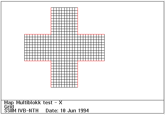
The grid, seen from above
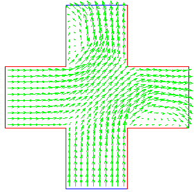
Velocity vectors, seen from above, level 6
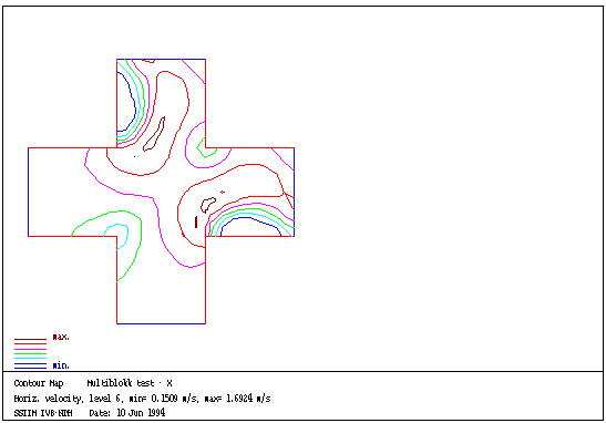
Contour map of horizontal velocity, level 6
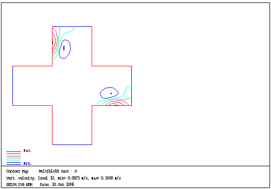
Contour map of vertical velocity, level 10
Y shaped channel
The files have extension .y. A channel branches in two at an angle of 45 degrees. The two branches have identical boundary geometry. The case was initially thought of being used for symmetry testing. However, the grid is not symmetrical, and therefore the flow field will not be completely symmetrical. This case is instead used for demonstrating sediment transport.
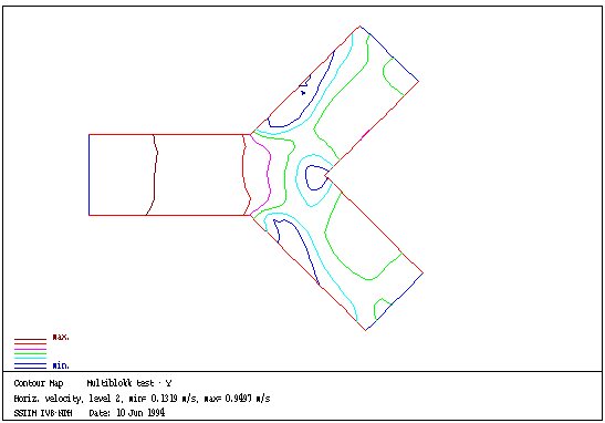
Contour map of horizontal velocity, bed level (level 2)
Curved channel
The files have extensions .svi. The channel is used for testing the programs ability to calculate the secondary flow pattern in a curved channel. It is also used for testing the routine that recalculates the water surface location based on the 3D flow field. The cross-sectional slope corresponds very well to theoretical solutions.
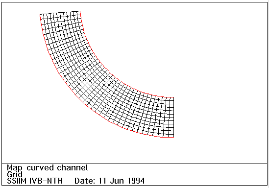
Grid of channel, seen from above
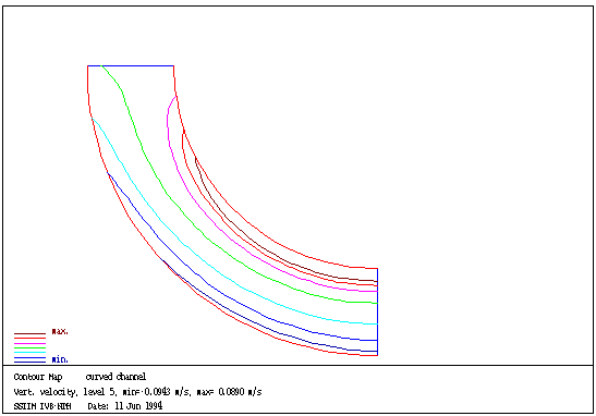
Contour map of vertial velocity, level 6
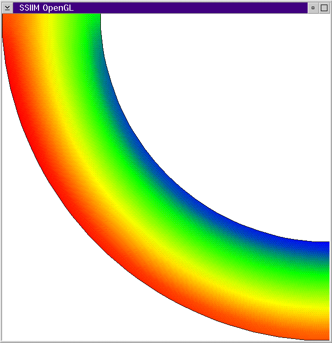
OpenGL color map of depth. Blue is minimum value and red is maximum value.
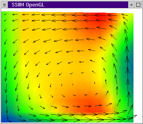
OpenGL color map of cross-secton at downstream end. The velocity vectors are parallell to the plane. The colors show velocity normal to the plane. Blue is minimum value and red is maximum value.
Fish farm tank
The files have extensions .kar. This case is used for demonstrating inflow and outflow at different locations in the geometry. The inflow is on one side, at 45 degrees to the wall. The outflow is at the bottom of the tank. The case is also used for demonstration of fish habitat. It is also suited for particle animation because the particle will move in a circular pattern. This case is further described by Olsen and Alfredsen (1994).
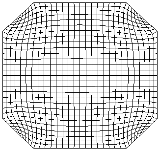
Grid, seen from above
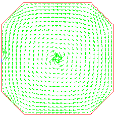
Velocity vectors at bed
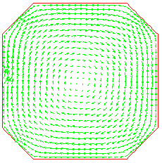
Velocity vectors at level 10
Reservoir sedimentation
The files have extension .res. This case is used for demonstration of trap efficiency calculation in a reservoir. It is a modified version of the Mae Tian reservoir calculation case from Thailand (Olsen and Melaaen, 1993 a,b). 8.3 cubic meters of water is flowing in through the reservoir. Several sediment sizes are used. The user can see the contour map of the bed levels, color map of the bed level changes, cross-section velocities and longitudinal profiles of the sediment concentration.
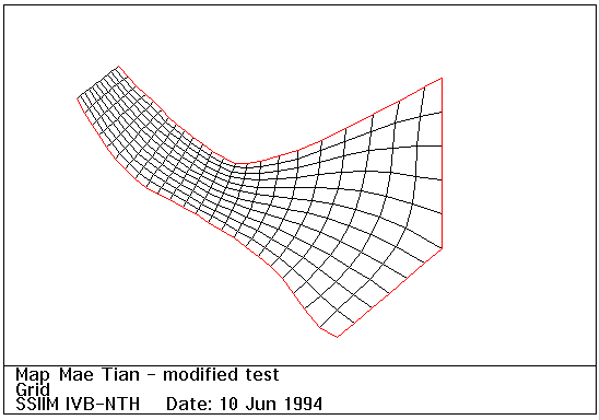
Grid, seen from above
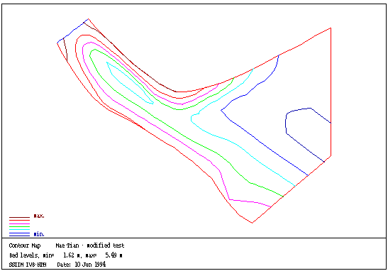
Contour map of bed levels
3D flood wave around building
The files have extension .wav. This example shows a flood wave in a 50 m long and 25 meter wide channel hitting a square building with sides 5 meters. The upstream water surface is 3 meters above the bed, and a water velocity of 3 m/s is in the inflowing water. The speed and the depth of the wave correspond to hydraulic formulas. The case is presented by Olsen (1994). Forces on the building are written to the forcelog file. A verification study for this example is presented by Lovoll et al (1995). More information
Turbidity current
The files have extension .tur. This example is a river flowing into a reservoir. The reservoir and the river has constant width. The inflowing water has a high sediment concentration (0.001 vol %), which causes a density current to form.
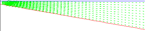
Velocity vector plot in a longitudinal profile after 15 seconds
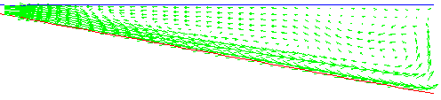
Velocity vector plot in a longitudinal profile after 255 seconds
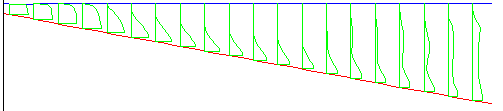
Concentrations a longitudinal profile after 255 seconds
Also note the reference by Olsen and Tesaker (1995). More information
Sand trap
The sand trap case is a verification case, where an 18 m long physical model of a sand trap were studied. The with of the sand trap was 1 m and it had a height of 1.5 m. The results from the physical model study compared fairly well with the results from the numerical model. For a further description of this study, see Olsen and Skoglund (1994) and Olsen and Chandrashekhar (1995). Example input files are not provided. Further description
Spillway
The files have extension .spi. A two-dimensional width-averaged spillway is calculated using the TFS routine. An almost horizontal water surface and water velocities of 1.0 m/s is used as initial values. Given a discharge of 1 qubic meters/second, SSIIM calculates the loation of the water surface and the flow field. The data set includes a timei. file, which tells SSIIM to write the upstream surface level for each time step. This makes it possible to calcualate the discharge coefficient. Compared with literature on design of dams, the coefficient is calculated with an error of 1.4 %. This case is also presented by Kjellesvig (1996).
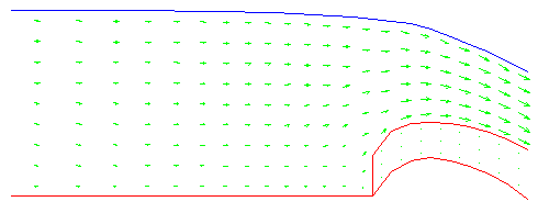
Flushing of a reservoir
A hydropower reservoir was filled with sediments to a given level. Then the sediments were flushed out by lowering the water level at the dam, allowing a water discharge with high velocity to flush out the sediments.This example was calculated by Olsen (1995), where it was compared with results from a physical model study.
The reservoir levels after one hour is shown above. The velocity vectors after one hour is shown below.
The reservoir levels after 2 1/2 hour is shown above. The velocity vectors after 2 1/2 hour is shown below.
Example of unstructured grid SSIIM 2.0
SSIIM version 2.0 is planned to have a more flexible grid, with multiple blocks, creating an unstructured grid. One procedure to generate the grid can be seen from the following figures.The grid editor is similar to the previous versions in the respect that points in the window from the geodata file is shown. Then the user can make several blocks, like shown below.
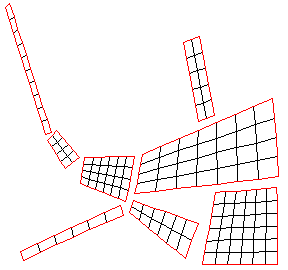
The sides of the grid are then connected.
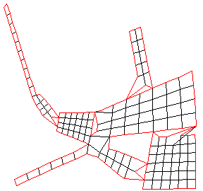
Each block is then adjusted according to the boundary.
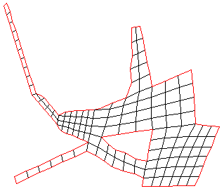
In the resulting grid, the blocks are connected.
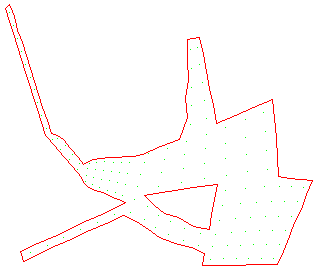
A bed interpolation routine gives a varying number of grid cells in the vertical direction, as shown in the longitudinal profile below.
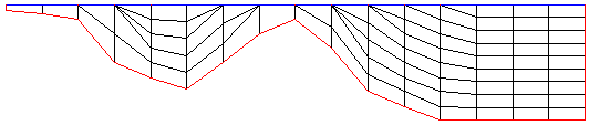
Literature
Ackers, P. and White, R. W. (1973) "Sediment Transport: New Approach and Analysis", ASCE Journal of Hydraulic Engineering, Vol. 99, No. HY11.Ashworth, R. (1993) "Renormalisation Group Turbulence Model", Eight International Conference on Numerical Methods in Laminar and Turbulent Flow, Swansea, UK.Blacker, T. D. and Stephenson, M. B. (1991) "Paving: A new approach to automated quadrilateral mesh generation", Int. Journal for Numerical Methods in Engineering, Vol. 32, pp 811-847.Chandrashekhar, J. (1994) "Numerical Simulation of Sediment Movement in Desilting Basins using SSIIM", M.S. Thesis, Division of Hydraulic and Environmental Engineering, The Norwegian Institute of Technology, Trondheim.Einstein, H. A. and Ning Chien (1955) "Effects of heavy sediment concentration near the bed on velocity and sediment distribution", UCLA - Berkeley, Institute of Engineering Research.Engelund, F. (1953) "On the Laminar and Turbulent Flows of Ground Water through Homogeneous Sand", Transactions of the Danish Academy of Technical Sciences, No. 3.Engelund, F. and Hansen, E. (1967) "A monograph on sediment transport in alluvial streams", Teknisk Forlag, Copenhagen, Denmark.Kjellesvig, H. M. (1996) "Numerical modelling of flow over a spillway", Hydroinformatics-96, Zurich.Kjellesvig, H. M. and St_le, H. (1996) "Physical and numerical modeling of the Himalaya Intake", 2nd Int. Conf. on Modelling, Testing and Monitoring for Hydro Powerplants, Lausanne, Switzerland.Lovoll, A., Lysne, D. K. and Olsen, N. R .B. (1995) "Three-dimensional modeling of flood waves around a structure", Submitted to the 26th IAHR Biennial Congress, London.Lovoll, A. (1996) "Hydrodynamic forces in unsteady open channel flow", Dr. Ing. dissertation, Department of Hydraulic and Environmental Engineering, The Norwegian University of Science and Technology.Lysne, D. K., Olsen, N. R. B., St_le, H and Jacobsen, T. (1995) "Withdrawal of water from sediment carrying rivers. Recent developments in planning and operation of headworks", International Journal on Hydropower and Dams, March.Mayer-Peter, E. and Mueller, R. (1948) "Formulas for bed load transport", Report on Second Meeting of International Association for Hydraulic Research, Stockholm, Sweden.Melaaen, M. C. (1992) "Calculation of fluid flows with staggered and nonstaggered curvilinear nonorthogonal grids - the theory", Numerical Heat Transfer, Part B, vol. 21, pp 1-19.Olsen, N. R. B. (1991) "A numerical model for simulation of sediment movements in water intakes", Dr. Ing. Dissertation, The Norwegian Institute of Technology, Trondheim.Olsen, N. R. B. and Melaaen, M. C. (1993a) "Numerical Modeling of Erosion around a Cylinder and Sediment Deposition in a Hydropower Reservoir", Eight International Conference on Numerical Methods in Laminar and Turbulent Flow, Swansea, UK.Olsen, N. R. B. and Melaaen, M. C. (1993b) "Three-dimensional numerical modeling of scour around cylinders", ASCE Journal of Hydraulic Engineering, Vol. 119, No. 9, September.Olsen, N. R. B., Jimenez, O., L_voll, A. and Abrahamsen, L. (1994) "Calculation of water and sediment flow in hydropower reservoirs", IAHR International Conference on Modeling, Testing and Monitoring of Hydropower Plants, Hungary. click here for more infoOlsen, N. R. B. and Alfredsen, K. (1994) "A three-dimensional model for calculation of hydraulic parameters for fish habitat", IAHR Conference on Habitat Hydraulics, Trondheim, Norway.Olsen, N. R. B. (1994) "SSIIM - A three-dimensional numerical model for simulation of water and sediment flow", Hydraulic Engineering Software V Vol. 2, Computational Mechanics Publications, ISBN 1-56252-290-6, (from HYDROSOFT-94, Porto Carras, Greece).Olsen, N. R. B. and Skoglund, M. (1994) "Three-dimensional modeling of water and sediment flow in a sand trap", IAHR Journal of Hydraulic Research, No. 6, Vol. 32.Olsen, N. R. B. and Tesaker, E. (1995) "Numerical and physical modeling of a turbidity current", 26th IAHR Biennial Congress, London.Olsen, N. R. B. and Oldervik, O. (1995) "Three-dimensional numerical modeling of water flow through a gate plug", 26th IAHR Biennial Congress, London.Olsen, N. R. B. (1995) "Numerical modelling of hydropower reservoir flushing", International Conference on Hydropower into the next Century", Barcelona, Spain.Olsen, N. R. B. and Stokseth, S. M. (1995) "Three-dimensional numerical modeling of water flow in a river with large bed roughness", IAHR Journal of Hydraulic Research, No. 4, Vol. 33.Olsen, N. R. B. and Chandrashekhar, J. (1995) "Calculation of water and sediment flow in desilting basins", 6th. International Symposium on River Sedimentation, New Delhi, India.Olsen, N. R. B. and Melaaen, M. C. (1996) "Three-dimensional numerial modeling of transient turbulent flow around a circular cylinder", 2nd. Int. Conf. on Modelling, Testing and Monitoring for Hydro Powerplants, Lausanne, Switzerland.Olsen, N. R. B. (1996) "Three-dimensional numerical modelling of local scour", Hydroinformatics-96, Zurich.Olsen, N. R. B. (1997) "Computational fluid dynamics as a tool for prediction of sedimentation and erosion in reservoirs", Q. 74 a), ICOLD Conference, Florence, Italy.Patankar, S. V. (1980) "Numerical Heat Transfer and Fluid Flow", McGraw-Hill Book Company, New York.Rhie, C.-M, and Chow, W. L. (1983) "Numerical study of the turbulent flow past an airfoil with trailing edge separation", AIAA Journal, Vol. 21, No. 11.Van Rijn, L. C. (1987) "Mathematical modeling of morphological processes in the case of suspended sediment transport", Ph.D Thesis, Delft University of Technology.Rodi, W. (1980) "Turbulence models and their application in hydraulics", IAHR State-of- the-art paper.Schlichting, H. (1979) "Boundary layer theory", McGraw-Hill.Sintic, A. (1996) "Numerical models for dam-break flood routing", MS Thesis, Institute of Hydraulic Engineering and Water Resources Management, University of Technolgy, Aachen, Germany.Vanoni, V., et al (1975) "Sedimentation Engineering", ASCE Manuals and reports on engineering practice - No54.Yang, T. C. (1973) "Incipient Motion and Sediment Transport", ASCE Journal of Hydraulic Engineering, Vol. 99, No HY10.The references by Olsen (1991), Chandrashekhar (1994) and Lovoll (1996) can be obtained by writing to:Department of Hydraulic and Environmental Engineering The Norwegian University of Science and Technology N-7034 Trondheim NorwayThe proceedings with reference by Olsen and Alfredsen (1994) can be obtained by writing to:SINTEF Civil and Environmental Engineering Klaebuvn. 153 N-7034 Trondheim NorwayThe thesis by Sintic (1996) can be obtained by writing to:RWTH Aachen Institut fur Wasserbau und Wasserwirtschaft Mies-van-der-Rohe-Str. 1 52056 Aachen Germany
![[IVB]](../../../../images/buttons/ivb_h.gif)
Copyright © 1998, Institutt for Vassbygging, NTNU

Fakultet
Inst. for vassbygging
Editor in charge: Astrid Kolberg
Webmaster: torove.leiknes@bygg.ntnu.no
Updated: 22 January 1998